Blog

  • How to Freeze a Row or Column in Excel

    How to Freeze a Row or Column in Excel

    Do you want to freeze a row or column in Excel? Do you find yourself constantly having to scroll back up to the top or to the left of the table to look at the headings? For example below, freezing the top row would be very useful because without row 1, we will not know what each number in Column B, C and D refers to.

    How-to-freeze-panes-Excel

    Freeze Top Row or First Column

    To freeze the top row:

    1. Scroll to the top
    2. Go to View tab
    3. Click on Freeze Panes
    4. Select Freeze Top Row

      Freeze-Top-Row-Excel

    We can now scroll down and Row 1 will always be visible, making it clear what each column is:

    Excel-Freeze-Top-Row

    And of course we could follow very similar steps to freeze the first column:

    1. Scroll to the left
    2. Go to View tab
    3. Click on Freeze Panes
    4. Select Freeze First Column

      Freeze-First-Column-Excel

    And now we can scroll to the right and Column A will always be visible, making it clear what each row is referring to:

    Excel-Freeze-First-Column

    Limitation: we cannot use both Freeze Top Row and Freeze First Column together. As soon as you select the other one, the first one disappears. Find out below how we can freeze both row and column.

    Freeze Row and Column

    There is of course a way to freeze both row and column in Excel. In fact the row and column do not have to be the top row or first column. We could freeze from Row 5 and from Column G if we wanted to. The easiest way would be to:

    1. Select the cell which is in the row and column we would like to freeze
    2. Go to View tab
    3. Click on Freeze Panes
    4. Select Freeze Panes

      Freeze-Row-and-Column-Excel

    And because C4 was selected in the picture above, Row 3 and Column B will now be frozen:

    Excel-Freeze-Column-Row

    Freeze Any Row OR Column

    In the section above, we went through how to freeze a row and column at the same time. In this section, we will look at how to freeze any row or column and they are not necessarily the top row or first column:

    1. Highlight the relevant row or column
    2. Go to View tab
    3. Click on Freeze Panes
    4. Select Freeze Panes

      Freeze-Any-Row-Column-Excel

    And as we can see, Column G is now frozen:

    Freeze-Any-Column-Row-Excel

    Similarly we can do the same thing with any row by first highlighting the relevant row.

    Unfreeze Panes

    Unfreezing pane is simple. We don’t even need to highlight the relevant column or row or have the cell selected. We could do so by:

    1. Go to View tab
    2. Click on Freeze Panes
    3. Select Unfreeze Panes

      Unfreeze-Panes-Excel

    Hotkeys for Freezing (or Unfreezing) Panes

    To freeze panes using hotkeys:

    • ALT > W > F > Choose the following:
    • F: to freeze or unfreeze pane
    • R: to freeze top row
    • W: to freeze first column

    And we recommend using the following hotkeys along with freezing panes:

    • Shift & space: highlight row
    • Ctrl & space: highlight column

    We hope you find this article useful. If you have any more questions regarding freezing panes in Excel, please leave a comment below and we will keep editing this article to make it more and more useful for everyone.

  • Dynamic Dropdown List in Excel

    Dynamic Dropdown List in Excel

    Dropdown List Dependent On Another Cell

    For a more complicated dropdown list, we can create dropdown list where the list changes depending on the value in another cell. In this example, we will create two dropdown lists. The first one is a simple dropdown list with the names of the countries (United States, Australia, England and Japan) and for the second dropdown list, the dropdown options will change depending on what is selected for the first one:

    1. Create Name Managers for the different lists by going to Formula tab and clicking on Name Manager

      data-validation-name-manager
    2. Go to Data tab at the top
    3. Click on Data Validation
    4. Allow: List
    5. For Source, there are two dropdown lists here. For the first list, select the first row ($A$1:$E$1) as the source:

      First list:
      data-validation-dropdown-list_

      For the second dropdown list, use the INDIRECT function and reference the cell where we have the first dropdown list:

      data-validation-second-dropdown-list_

      And this is the final result:
      data-validation-two-dropdown-lists

    With this logic, we can keep going and create another dropdown list that is dependent on the second dropdown list and so on…

    We hope you find this article useful. If you have any more questions on creating a dynamic dropdown list in Excel, please leave a comment below and we will keep editing this article to make it more and more useful for everyone.

  • Searching for a Value that has Multiple Entries in the Table

    Searching for a Value that has Multiple Entries in the Table

    The VLOOKUP function searches for the lookup_value in the leftmost column in the table_array and stops when the first match is found. But what if there are multiple entries in the table?

    Have a look at an example below:

    multiple-entries-in-table

    There are multiple “Kate N”s in the company. Using VLOOKUP, you will only get Start Date or Employee Number for the first “Kate N” in the list. So how can we get the full list of Start Dates or Employee Numbers for all “Kate N”s.

    FILTER Function in Excel

    The FILTER Function is perfect for the occasion and is simple to use.

    The FILTER function is:

    • =FILTER(array, include, [if_empty])

    • array: the range of cells you want returned
    • include: the value to search for and the range of cells to look for that value
    • [if_empty]: what should the function return if nothing can be found

    In order words, with the FILTER function, we first enter the range of cells which we want Excel to possibly return. And then we specify what the lookup value is and the range of cells Excel should look for that value. In the example below:

    • array: Employee Numbers which is the C2:C34 range
    • include: the value to search for which is “Kate N” in E2 and we want Excel to look for that in the Staff Directory list which is the A2:A34 range

    Filter-function-Excel

    In the example above, we did not use [if_empty]. It is an optional field. It specifies what should be returned if the lookup value cannot be found. For example below, we can specify “Not Found” to be returned if staff’s name in E2 is not in the Staff Directory list in column A.

    If you choose to not use the [if_empty] field, you will get a #CALC error when the lookup value cannot be found.

    Right to Left (Unlike VLOOKUP)

    Another advantage the FILTER function has over VLOOKUP is that VLOOKUP must start searching for the lookup value in the leftmost column and can only return a value on the right side of that value in that row. With FILTER function, you can move start from the right and look for a value in the right side column and have Excel return a value on the left:

    Filter-function-Excel-right-to-left

    This means we could specify an Employee Number and find the name of the staff without having to rearrange the columns in the table. This would not be possible with VLOOKUP.

    #SPILL Error in FILTER function

    #SPILL error appears with FILTER function when Excel wants to return multiple results but the cells below are not empty. In the example below, there are four “Kate N”s and hence there are four Employee Numbers the FILTER Function would like to return. But F3:F5 already have data in those cells (“A”, “B” and “C”). Once “A”, “B” and “C” are removed, #SPILL will disappear.

    Filter-function-Excel-spill-error

    We hope you find this article useful. If you have any more questions on this topic, please leave a comment below and we will keep editing this article to make it more and more useful for everyone.

  • REPLACE Function – Changing Existing Text with New Text

    REPLACE Function – Changing Existing Text with New Text

    In this article, we will have a look at the REPLACE function. We will look at how to use this function to change existing text in a string with new text. We will also look at how the REPLACE function is different to the SUBSTITUTE function and when to use each one.

    REPLACE Function

    The REPLACE function requires 4 variable input. Before we start explaining what each field means, it is best to think of the REPLACE function as first removing a portion (or all of the) existing text and then replacing it with new text :

    • Old_text: this is the current text/string or cell reference we would like to edit
    • Start_num: this is the starting position in the old_text from which current text should be removed. For example if we put 4, then Excel will remove the existing text from the 4th character
    • Num_chars: from the start_num position, how many characters should be removed?
    • New_text: after removing “num_chars” number of characters starting from the “start_num” position, what should be replaced?

    It is important to note that the number of characters in the “new_text” does not need to match the “num_chars”. This means you could remove 3 characters in the current “old_text” and replace it with a “new_text” that is 2 characters or 9 characters.

    Let’s go through a simple example:

    Replace-Function-Example

    =REPLACE(A2,1,7,”Team-C-“)

    In this case, we have a list of people from Team A and from Team B. And we are merging the two teams to become Team C. For each row, first we are removing 7 characters (num_chars: 7) starting from the first position (start_num: 1) and we are replacing it with “Team-C-” as the new text (“new_text”).

    Here’s another example:

    Replace-Remove-Strings-Excel

    =REPLACE(A2,1,8,””)

    Here we simply want to remove the first 8 characters so we are left with the name in each cell. In this case, we are removing the first 8 characters and replacing it with…nothing as the new text (“”).

    And finally we have a slightly more complex formula where we combine the FIND function with REPLACE function:

    Replace-Find-Remove-Strings-Excel

    =REPLACE(A2,1,FIND(” “,A2),””)

    The example is only a little more complex because the number of characters to remove in each row is different. But we do know that the two words are separated by a space. So we want to remove all characters up to the space. This means we just need to find the position of the space which we can do with FIND function: FIND(” “, A2). After that, it becomes a very similar example as the previous one – starting from 1 position, we remove nth number of characters depending on where the space is and we replace it with “” (nothing).

    REPLACE Function vs SUBSTITUTE Function

    The REPLACE function and the SUBSTITUTE function serve a very similar purpose, if not the same. In fact, if we look at the definitions of each function in Excel, they are hardly distinguishable:

    Definition-Replace-Substitute-Functions-Excel

    The difference lies in how each one is used:

    • REPLACE function removes existing strings with users specifying the starting position and the number of characters to be removed
    • SUBSTITUTE function removes existing strings with users specifying specifically what character(s) to remove

    That means if you know exactly what you are removing from the original text, you should use the SUBSTITUTE function. If you only know the position from which you want to remove and replace in the original text, you should use the REPLACE function.

    Here’s an example to illustrate the difference:

    Replace-Substitute-Examples-Excel

    In the example of the left, we want to remove the first 8 characters for every row so the REPLACE function is more suitable. With the second example, we don’t necessarily want to make any changes in every row. We only want to change all the “HFI” with “Anonymous”. And in this case, SUBSTITUTE function is more suitable because all the other strings that do not have “HFI” will remain unchanged.

    We hope you find this article useful. If you have any more questions regarding replacing existing texts in Excel, please leave a comment below and we will keep editing this article to make it more and more useful for everyone.

  • How to Change and Substitute Specific Text in Excel

    How to Change and Substitute Specific Text in Excel

    There could be various reasons why we need to change and substitute certain text in a cell. We have touched on this previously when needed to take out certain part of a string in a cell (How to Extract Part of a Text in Cells). You could be doing this to clean up data or simply to help with reporting. Whatever reason it is, in this article we will go through two ways on how to change and replace specific text in Excel.

    Find and Replace

    We will first go through the more simple way of doing this. And that is to use the Find and Replace function in Excel. The hotkey for it is CTRL & H. Alternatively we can find it in the Home tab, in the Editing section > Find & Select > Replace…:

    Find-and-Replace-Excel

    Change-and-Replace-Excel

    Here we could find and replace any text we would like. If no cell is selected, the “Find and Replace” will apply to everything in the worksheet. However we can have selected cells highlighted and only replace specific texts for those certain cells.

    For example below, we only have A2:A10 highlighted and we will replace all “PCS” to “MQCS”:

    Find-and-Replace-Specific-Cells-Excel

    Click “Replace All”:

    Texts-Replaced-Excel

    Simple to use but has certain limitations:

    • In a cell where the text appear in multiple instances, we cannot specify whether we only want to replace the first or second or third text. E.g. in the example above, we could not use “Find and Replace” to only replace the second dash
    • Not being in a formula or function also means we cannot wrap this with another formula. And to not change the original data, we would have to copy and paste data into another location, do a “Find and Replace” and then apply another formula/function to it. That is just not the most efficient way to use Excel.

    With that in mind, we will now explore another method to change and replace specific texts in Excel. This time, with a built-in Excel function.

    SUBSTITUTE function

    There is a built-in function in Excel called SUBSTITUTE and its purpose is to:

    • Replace existing text in a string with new text

    This function requires 3 mandatory inputs and 1 optional variable:

    • The text or cell reference: this can also be an array in which case the results will spill into adjacent cells
    • Old text: the existing text in the string to be replaced
    • New text: what the old existing text should be placed with
    • [Instance_num]: this is the optional input. It is the variable which allows us to choose, in cases where the existing text appears in multiple occasions, which existing text to replace in the string. By default if this is blank, all of them will be replaced.

    Using the above example again, with the SUBSTITUTE function, we can change and replace the second dash “-” with another character and leave the first one unchanged:

    SUBSTITUTE-Function-Excel

    =SUBSTITUTE(A2, “-“, “@”, 2)

    Here we are changing the text in cell A2. We are changing “-” to “@” and only the second instance “-” comes up. Note that if we put a number for [instance_num] that is more than the number of times the old existing text appears in the cell, Excel will just not change and replace any of them. And if we put 0 or a negative number, we will get #VALUE error.

    Why Is This Useful?

    There could be a number of reasons why this would be useful. One thing we can agree on is that it is definitely more flexible than “Find and Replace” or CTRL & H. With the example above, after replacing the second dash with “@”, we can now wrap the SUBSTITUTE function inside a FIND function and this will help us find where the second dash (now replaced with “@”) was:

    • =FIND(“@”,SUBSTITUTE(A2,”-“,”@”,2))

    And with that, we can now use the RIGHT function to extract the names of all the employees in the list:

    • =RIGHT(A2,LEN(A2)-FIND(“@”,SUBSTITUTE(A2,”-“,”@”,2)))

      Extracting-Names-RIGHT-Function-Excel

    We hope you find this article useful. If you have any more questions regarding changing and replacing certain texts in Excel, please leave a comment below and we will keep editing this article to make it more and more useful for everyone.

  • How to Compare Two Columns

    How to Compare Two Columns

    There are many different ways to compare two columns. And it depends on how we want to do the comparison? Do we want to simply see if item in one column is in the second column? Do we want to count how many rows have different items? Do we want to specify which rows have the same items and which don’t? In this article, we will go through as many as of these scenarios possible.

    Comparing Line By Line

    Comparing-Two-Columns-Data

    When we have two columns of data, one way to compare the two columns could be to simply see if the names/items for each row match. In this case, we can do so with an IF function:

    Comparing-Two-Columns-IF-Function-Excel

    =IF(A2=B2,”Y”,”N”)

    And then to highlight the rows that do not match, we can apply filter (CTRL & Shift & L):

    Comparing-Two-Columns-IF-Function-Filter-Excel

    In the example below we will look at how we can specify what the difference is.

    Specifying What The Difference Is

    What if instead of simply stating each row matches or not, we want to specify what the difference is? We can do that with a slight variation to the IF function:

    Comparing-Two-Columns-IF-Function-Specify-Difference-Excel

    =IF(A2=B2,”Match”,“Column A -“&A2&” and Column B -“&B2)

    All we have really changed here in the IF function is what the function should return should Column A not match Column B. And instead of simply returning “N”, we have a bunch of strings that are concatenated together by “&”.

    We can easily edit the formula to have it return different values in various different formats. If you have any particular format you would like to see and you are stuck, feel free to leave a comment below!

    Total Number of Lines That Are Different

    Now what if we don’t care which rows match and which ones don’t and we only want to know the total number of rows that match and the total number of rows that don’t? Well here it is:

    Comparing-Two-Columns-Totals-Excel

    =SUM(IF(A2:A34=B2:B34,1,0))

    =SUM(IF(A2:A34<>B2:B34,1,0))

    To break the first formula down, what we have is:

    • If A2 equals B2 then Excel will return 1. If they are not the same, then return 0. By putting the entire arrays in the formula (A2:A34 and B2:B34), we can have Excel compare A2 with B2, A3 with B3, A4 with B4 and so on… And by nesting the whole formula within a SUM function, Excel adds all the 1s and 0s together.

    The second formula is very similar except this time we are changing the logical test in the IF function. This time we don’t want the two columns to equal (=) each other but we want 1 to return when they are different (<>).

    What is in First Column but not in Second Column?

    In the section above, we were comparing the two columns row by row. But what if we simply want to see if names/items in the first column is or is not in the second column? So in this case, the order of the list does not matter.

    Excel-COUNTIF-Comparing-Two-Columns

    =IF(COUNTIF($B$2:$B$34,A2)>0,”Y – In Column B”,”N – Not In Column B”)

    We’ve put the list in Column B in a random order. To break the formula down, we are using COUNTIF function to see if each name/item in Column A is in Column B. As long as Excel returns a result that is more than 0, it will return “Y – in Column B” otherwise it will return “N – Not in Column B”.

    Once again we can use filter to see which items are not in Column B:

    Filter-Not-In-Second-Column-Excel

    How Many In First Column Can Be Found in Second Column?

    In this scenario we simply want to know the total number of names/items that appear and not appear in Column B:

    Total-In-Column-B-Excel

    =SUM(IF(COUNTIF($B$2:$B$34,A2:A34)>0,1,0))

    =SUM(IF(COUNTIF($B$2:$B$34,A2:A34)=0,1,0))

    Breaking the first formula down, we are using COUNTIF to see if A2 is in Column B. If the result is more than 0, then Excel will return 1 otherwise it will return 0. By putting the criteria as an array A2:A34, we are getting Excel to run this COUNTIF from A2 down to A34. Without the SUM function, Excel will list down all the results (1 or 0). By nesting this into a SUM function, Excel will add all results (1s and 0s) together and return the total.

    The second formula is very similar, except we want COUNTIF to return 0. This will indicate to us the name/item in Column A is not in Column B. The best way to check our work is that the total of these two results (21 and 12) add up to the total number of names/items in Column A.

    Have we missed anything? How would you like to compare two columns? Leave us a comment to let us know what you need and we will add it onto this article!

  • How to Calculate Sum or Count Based on Cell Colors

    How to Calculate Sum or Count Based on Cell Colors

    In this article we will do a step by step guide on how to add up values based on cell colors. And then we will go through how to count the number of cells that are of a particular color. We will be doing so using Visual Basic for Applications (VBA). However this method is not without its limitation. Before we end this article, we will explain what the limitation is and provide tips on how to work around it.

    Before we start, as we mentioned, we will be using VBA to do this so please make sure VBA is enabled in your Excel file.

    Calculate SUM Based on Cell Colors

    To calculate sum of a set of values based on colors of the cells, we will be creating very own user-defined function. This is something we have gone through in a previous article: User-Defined Functions – Writing Your Own Functions in Excel.

    To begin:

    1. Go to Developer tab
    2. Click on Visual Basic
    3. Click on Insert at the top
    4. Select Module
    5. Copy and paste the following code into the module:
    Public Function SumByColor(colorcell, cellrange) As Double

    WhatColor = colorcell.Interior.Color
    x = 0

    For Each coloredcell In cellrange
    If coloredcell.Interior.Color = WhatColor And IsNumeric(coloredcell) = True Then
    x = x + coloredcell
    End If
    Next coloredcell

    SumByColor = x

    End Function

    The first step to writing any user-defined functions is always to always have a name for the function and also consider what variables/fields do we require from the users each time they use this function. In this case, we named the function SumByColor (you can call it something else) and there are two inputs we require each time:

    1. The cell that has the color which we want to reference for this function: colorcell
    2. The range of cells which the function will check if the cell color is colorcell (from above): cellrange

    Now let’s explain the codes step by step:

    1. First off, we need to let this function know the color it is looking for in the range of cells. And that is what the first variable or field is for: colorcell. Inside the module, we first create a variable: WhatColor – this variable stores the color index of the cell color for colorcell:

      WhatColor = colorcell.Interior.Color
    2. Next we create another variable called x – this variable will keep adding a new value onto itself if its cell color matches with WhatColor. At the start of this function, we will set:

      x = 0

      This is because at this point, we haven’t checked any cell in cellrange against WhatColor yet.
    3. The next step is to run a loop. The loop will go through each cell in the cellrange specified in the function:

      For Each coloredcell In cellrange

      Note that the variable coloredcell can really be called anything. It’s just another variable we’re creating for this loop.
    4. For each cell in the cellrange, there are two checks we want to do: 1) if the cell color matches WhatColor and 2) if the value in the cell is a number. If both are true, then we will add the value in that cell to x. And this new value becomes our new x:

      If coloredcell.Interior.Color = WhatColor And IsNumeric(coloredcell) = True Then
      x = x + coloredcell
      End If

    5. Once all the cells in cellrange is looped through, the final x will be the sum of all the values that are in cells of a particular color we want. And this is what we want the function to return:

      SumByColor = x

    Let’s test this out. We named our user-defined functions SumByColor so we should be able to see the function now if we enter it into a cell:

    User-Defined-Functions-Sum-Based-On-Colors-Excel

    There are two fields required: 1) colorcell and 2) cellrange:

    Sum-Based-On-Cell-Colors-Excel

    =SumByColor(C2,$A$1:$A$97)

    For each formula, we first reference the cell on the left (in the first formula: C2). This tells the function what color we are looking for. Not that we need to know but Excel looks at the color of this cell and stores the color index as WhatColor. And then Excel loops through each cell in range A1:A97. For each cell which has color matching WhatColor, the value gets added onto a variable called x. And at the end of the loop, the function returns the value of x.

    Note that the “If IsNumeric(coloredcell) = True” is important because otherwise we could be asking Excel to do an addition with non-numerical values, in which case Excel would return #VALUE. But with this condition added to the IF statement, if Excel recognizes that the value is not numerical (even if the color matches), it will skip over this value:

    Sum-Non-Numerical-Values-Excel

    COUNT Number of Cells With A Particular Color

    Next we will look at how to create a user-defined function that can count the number of cells that are filled with a particular color. Again, first thing to do would be to make sure our Excel file is macro-enabled.

    Secondly we will need to think of a name for our function. In this case, we will call our function: CountByColor. Essentially you can give your function whatever name you want (except one that is already used by a built-in function in Excel) but it is good practice to choose a name that actually makes sense to you and to everyone who will be using your Excel file.

    Similar to calculating the sum of values based on the cells’ colors, we need the exact same variables/inputs for this function:

    1. The cell that has the color which we want to reference for this function: colorcell
    2. The range of cells which the function will check if the cell color is colorcell (from above): cellrange
    Public Function CountByColor(colorcell, cellrange) As Integer

    WhatColor = colorcell.Interior.Color
    x = 0

    For Each coloredcell In cellrange
    If coloredcell.Interior.Color = WhatColor Then
    x = x + 1
    End If
    Next coloredcell

    CountByColor = x

    End Function

    Now let’s explain the codes step by step:

    1. First off, we need to let this function know the color it is looking for in the range of cells. And that is what the first variable or field is for: colorcell. Whatever color this cell is filled with, this function will match every cell in the second variable against this color. And we create a variable WhatColor to store this color index:

      WhatColor = colorcell.Interior.Color
    2. Next we create another variable called x – this variable will keep adding one to itself if the cell color matches with WhatColor. At the start of this function, we will set:

      x = 0

      This is because at this point, we haven’t checked any cell in cellrange against WhatColor yet.
    3. The next step is to run a loop. The loop will go through each cell in the cellrange specified in the function:

      For Each coloredcell In cellrange

      Note that the variable coloredcell can really be called anything. It’s just another variable we’re creating for this loop.
    4. For each cell in the cellrange, we want to check if the cell color matches WhatColor. If it does, then we will add one each time to x:

      If coloredcell.Interior.Color = WhatColor Then
      x = x + 1
      End If


      Optional: Note that in the SumByColor function, we had the additional check to make sure the cell value is numerical. We didn’t do that in this case since we are not adding any values together. But theoretically, we could add more conditions. E.g. we could make sure the cell is not blank by adding:

      And Len(coloredcell)>0

      In which case, the If statement becomes:

      If coloredcell.Interior.Color = WhatColor And Len(coloredcell) > 0 Then
    5. Once all the cells in cellrange is looped through, the final x will be the total number of cells that are filled with WhatColor. And this is what we want the function to return:

      CountByColor = x

    Let’s test this out. You should now be able to see a CountByColor function:

    User-Defined-Functions-Count-Based-On-Colors-Excel

    There are two fields required:

    Count-Based-On-Cell-Colors-Excel

    We first reference the cell on the left (in the first formula: C2). This tells the function what color we are looking for. Excel then stores this color index as WhatColor and then it loops through each cell in range A1:A22. For each cell which has color matching WhatColor, the variable x adds one to itself. And at the end of the loop, the function returns the value of x.

    As mentioned above, we could add more conditions depending on what we need. For example besides from the color of the cell, we could also test whether the value is numerical, or we could test whether the value is over 1000.

    What To Be Mindful Of…

    Before we end the article, let’s go through what we need to be mindful of with these two user-defined functions above because there are key two limitations:

    1) When Does The Function Recalculate Itself?

    One thing to keep in mind is whether the function recalculates itself automatically and when. In Excel, if in a function you reference another cell or range of cells and let’s say the value in those referenced cell(s) changes, the value from your function will update itself automatically.

    Rest assured this is the same with the user-defined functions we just created. However from Excel’s perspective, changing a background color of a cell is not the same as updating/changing a value in a cell. Simply put, changing a cell color is not a catalyst for Excel to recalculate its functions and formulas. This means if you add a number into a cell and then change the color of the cell, the two user-defined functions will not pick them up (at least not until a value is updated somewhere in the worksheet that will trigger Excel to recalculate all its functions and formulas).

    Workaround:

    Instead of entering a value into the cell and then changing the color of the cell, do it the other way around. You will need to first change the color of the cell and then update value in it. Simply put, it is the updating of the value that triggers Excel to recalculate all the functions and formulas. So by updating the value after changing the cell color, the user-defined functions will be updated.

    2) This Does Not Work With Conditional Formatting

    Unfortunately this just doesn’t work with conditional formatting. To illustrate this, we created another user-defined function: WhatColorCell. This function checks the color of a particular cell and returns the color index:

    Public Function WhatColorCell(checkcolor) As Double

    CellColor= checkcolor.Interior.Color
    WhatColorCell = CellColor

    End Function

    In the examples below, we used this function on three different cells 1) the first one is filled with red, 2) the second has conditional formatting such that if the cell value is over 200, it will be formatted as red and 3) the cell has no color filled at all:

    Conditional-Formatting-Color-Cell-Excel

    As we can see, even with conditional formatting, the color index returned is the same for 2 & 3. From Excel’s perspective, a conditionally formatted cell has the same color index as a cell with no filled color. That is, provided of course the conditional formatted cell was not previously filled with a color.

    We hope everyone finds this article helpful. If you have any questions regarding this article or if you have any suggestions on how we can change it and what we can add, please leave a comment below!

  • Difference Between Absolute and Relative Cell Referencing

    Difference Between Absolute and Relative Cell Referencing

    In Excel we often reference another cell or a range of cells in a function or formula. And we drag the formula down the row so we don’t type the same formula again and again. Inevitably there will be times we want Excel to lock in a particular cell or range and there will be times we want Excel to keep shifting the cell up or down or across as we drag the formula. This is where absolute and relative cell referencing are useful.

    Absolute Cell Referencing

    • Absolute Cell Referencing is when we lock in a particular cell or range such that even when we drag the formula across to other cells, the cell or range referenced in the formula does not change.

    How Do We Do This?

    We do this by adding “$” signs in front of the referenced cell or range in the formula. As an example, we can lock in A1 in the formula below:

    absolute-cell-referencing-Excel

    By adding “$” to A1, we lock in A1 so that when we drag the formula down, Excel will continue to calculate =SUM($A$1). Without the “$”, by default, Excel would shift the cell down so that C2 will be =SUM(A2), C3 will be =SUM(A3) and so on.

    Tip: you don’t need to type the $ every time. The short key for absolute cell referencing in Excel is F4. By pressing F4, Excel will automatically put $ around the cell or range referenced.

    You can see above there are two “$”s with $A$1. This is because you can specify whether you want to absolute reference the column or the row. In the example above, if we have $A1 instead of $A$1, because Row 1 is not locked in, when we drag the formula down, Excel will shift the cell down to $A2, $A3, $A4 and so on. And because the formulas are all in Column A, absolute referencing Column A in the formulas is actually not very useful at all.

    Relative Cell Referencing

    Have you ever copied a cell because it has a certain value in it but when you paste it in another cell, the value is completely different in the pasted cell?

    • Relative Cell Referencing is the opposite of absolute cell referencing and this is by default in Excel. It means when you first reference a cell or range in your current cell, Excel takes into account the location of that referenced cell or range in relation to the current cell you are typing in.

    As mentioned this is the default in Excel. As an example below, if we reference A1 in C1, as we drag the formula down, Excel will automatically shift the referenced cell down by one each time. Such that in C2, the formula becomes =SUM(A2).

    Relative-Cell-Referencing-Excel

    This applies to more than dragging formulas. As an example below, we put “123” in Cell A1 and in Cell C3, we put “=A1”.

    Excel-Relative-Cell-Referencing-No-Formula

    By doing this, Excel has recognized that we are reference a cell that is “two cells to its left and two cells above”. If we now copy and paste Cell C3 and paste in Cell E5, Excel will recognize that we want to reference a cell that is “two cells to its left and two cells above” – in this case C3.

    Relative-Cell-Referencing-another-cell-Excel

    Of course we need to keep in mind this is not restricted to what we’ve put in A1. If we now put in “Andrew” in another random cell, say Cell B6, and we copy Cell C3 or Cell E5 and paste it in Cell D8, Cell D8 will still pick up whatever is in Cell B6 because it is two cells to its left and two cells above:

    Using Absolute and Relative Cell Referencing in the Same Formula

    Of course we can use both absolute and relative cell referencing in the same formula in Excel. We do that a lot in COUNTIF function where we absolute reference the criteria_range and use relative referencing for the criteria. We will go through an example below. Here we have monthly revenues listed down and in Column D, we want to calculate year-to-date revenue. This means for January, the YTD revenue will just be January. For February, it will be January and February. For March, it’ll be January to March and so on:

    Absolute-and-relative-cell-referencing-Excel

    In essence, we are calculating the total revenue from January to current month. This means we want to absolute reference January but relative reference current month because current month changes every month. By typing for January:

    • =SUM($B$1:B1)
    • We are essentially just putting January revenue in D1. But as we drag the formula down, $B$1 remains as the first cell in the range but the second cell – which is relative referenced: B1 – will keep shifting down to B2, B3, B4 and so on accordingly each time.
  • Rounding Numbers and Decimals in Excel

    Rounding Numbers and Decimals in Excel

    If you are interested in rounding numbers and decimals in Excel, you’ve found the right article. In this article, we will go through how to round decimal numbers up and down, specifying how many decimal places we want and also rounding numbers to the nearest multiples.

    Rounding Decimals – ROUND, ROUNDUP and ROUNDDOWN functions

    There is a few Excel built-in functions that can be used to round up/down decimals and specify how many decimal places we want. Instead of going through them separately, we will explore them together in this section so we can see the differences and know when to use each one. There are three functions:

    • ROUND, ROUNDUP, ROUNDDOWN

    With each function, there are two variables that needs to be entered: 1) the number that needs rounding up/down and 2) the number of decimal places to be rounded to. Here’s the difference between the three:

    1. ROUND: this function runs decimals up and down in accordance with the standard mathematical rules. For numbers 1 to 4, Excel would round the decimal down. For numbers 5 to 9, Excel would round the decimal up.
    2. ROUNDUP: this function is different to above because it will always round a decimal up. If we use ROUNDUP with 1.51 and round to one decimal place, it will return with 1.6.
    3. ROUNDDOWN: this function is the exact opposite of ROUNDUP. It will always round a decimal down. For example if we use ROUNDDOWN with 7.99 and round to one decimal place, it will return with 7.9.

    Which one you use will depend on the situation. An example of where ROUNDUP could be useful would be parking fees in a carpark. We often pay for parking by the hour and as soon as we are one minute past the hour, we will need to pay for an extra full hour. For example, if you park in a carpark for 3 hours and one minute, you don’t pay for 3 hours and one minute, you pay for 4 hours. It rounds up.

    Let’s have a look at a few examples here. The first picture below, we are using ROUND, ROUNDUP and ROUNDDOWN with the decimal number on the far left and for each function, we are rounding to two decimal places:

    Rounding-decimals-2-Decimal-places-Excel

    Hopefully laying the functions and results side by side, you will be able to clearly see the differences. ROUND function should operate mathematically as we would all expect. With ROUNDUP, regardless what the 3rd decimal place is, the second decimal place will always go up by one. With ROUNDDOWN, regardless what the 3rd decimal place is, the second decimal place will always remain unchanged.

    Here’s another example. In this case, we want 0 decimal place:

    Rounding-decimals-whole-numbers-Excel

    The logic is the same. With ROUNDUP, regardless what the first decimal place is, it will always round the whole number up by one. With ROUNDDOWN, regardless what the first decimal place is, the whole number will always remain unchanged.

    Rounding Numbers to a Particular Multiple

    In this section we will go through how to round numbers to a particular multiple. The function is MROUND. There are two variables required: 1) the number that needs rounding up/down and 2) the multiple to which the number is to be rounded to. We could specify any number and multiple and MROUND would round the number to the nearest multiple – up or down depending on which is closer.

    In the examples below, for each number on the left, we are rounding it to the nearest multiples of 5s. For 1946, it is closer to 1945 than it is to 1950 so Excel returned 1945:

    Rounding-Numbers-Multiple-Excel

    And if the number is right in the middle between the two nearest multiples, it will be rounded up. In this example we are rounding each number to an even number. And in both cases, the number is rounded up to the next even number:

    Excel-Rounding-to-Even-Numbers

    Choosing to Round Up or Down to a Particular Multiple

    In the section and examples above, we can’t choose whether to round the number up or down. Excel does so for us depending which multiple is closer or in the situation where the number is in the middle, it rounds up to the higher multiple. What if we want to choose to always round up (or down) to the higher (or lower) multiple?

    There is no built-in Excel function for this but the formula is not too complex:

    • Rounding Up:
      • = ROUNDUP(A2/n, 0) * n
      • (n: the multiple)
    • Rounding Down:
      • = ROUNDDOWN(A2/n, 0) * n
      • (n: the multiple)

    The logic is simple. With rounding up, whatever the number is, we first divide it by the multiple. If it is divisible then no rounding is required. If it is not divisible, there will be a decimal. And from what we went through with ROUNDUP function above, if we set decimal place to 0, the number will always be rounded up to the next whole number. For example: 22.3 will become 23, and then we can multiply 23 by the multiple. This will always round the number up to the next multiple.

    Same logic with ROUNDDOWN. Whatever decimal we get, the number will remain unchanged. For example: 122.43 becomes 122, and then we multiple 122 by the multiple. This will always round the number down to the lower multiple.

    See example below:

    Rounding-numbers-up-down-multiples-Excel

  • Using Check Boxes in Excel

    Using Check Boxes in Excel

    Check boxes in Excel are a useful tool in creating checklists or to-do lists. They are simple to use. Everyone knows how to use a checklist. Users only have two options: tick the checkbox or deselect it. In this article, we will go through step by step how to add check boxes in Excel. And then more importantly we will look at how we can use the results in the checkboxes. This includes using formulas to calculate the results, setting conditional formatting based on check boxes and lastly how to add VBA/Macro into check boxes. However before we start, let’s look at the differences between check boxes and radio buttons because they are different in Excel and should be used differently.

    Check Boxes vs Radio Buttons – When To Use Each One?

    In the Developer tab, under the Controls Section, there is a list of Forms Controls we could insert. Two of which are check boxes and option button (radio buttons). At first glance just by looking at them, the only difference is that one is shaped as a box and the other is shaped as a button. What’s the difference and when should we use each one?

    Check boxes:

    • Users can select as many check boxes as they want
    • Users can deselect any or all of the check boxes

    Radio buttons:

    • Users can only select one radio button at a time
    • Selecting one button will automatically deselect all the other buttons
    • Unless we go into Format Control to deselect a radio button, one button must be selected at all times within a group

    Simply put, check boxes should be used if you want to be able to select multiple options. And radio buttons should be used if you only want to select one option at a time. In this article, we will only go through check boxes in Excel.

    How To Add Check Boxes?

    First of all, to be able to insert check boxes, we need to access the Developer tab and make sure the Excel file is saved as macro-enabled. For more instructions on that, please click here.

    Once we can see the Developer tab, we can insert a check box by:

    1. In the Controls section, click on Insert
    2. Select Check Box:

      Insert-Check-Boxes-Excel
    3. Click on anywhere in the worksheet and a check box will be inserted

    To generate more check boxes, we could either:

    1. Copy the check box and paste as many as we want
    2. Align the current check box into a cell and drag the cell down or across as though we are copying a formula:

      More-Check-Boxes-Excel
      Many-Check-Boxes-Excel

    Formatting Check Boxes

    By default, after inserting a check box, this is what the check box will look like:

    Default-Check-Box-Excel

    In most cases, we will need to do some formatting with it. That is of course unless we just want to leave it as “Check box 1”, “Check box 2”, etc. To edit the wording next to the check box:

    1. Right-click on the check box
    2. Select Edit Text

      Excel-Edit-Text-Check-Box
    3. Edit text as you wish. Note that you could have no text at all next to a check box:

      No-Text-Check-Box-Excel

    To select and move the check box around:

    1. Right-click on the check box to select it and then move it around, or;
    2. Hold the CTRL key and click on the check box. Then we can move it around

    Linking A Check Box To A Cell

    Before going through how to apply formulas to check boxes or conditional formatting, we first need to know how to link a check box to a cell. By linking a check box to a cell, we can then use formulas to reference that check box by referencing the cell because they are now linked:

    1. Right-click on the check box
    2. Select Format Control:

      Format-Control-Excel-Check-Boxes
    3. Click on the Control tab
    4. In the Cell link field, enter the cell you would like to link the check box with

      Excel-Linking-Cells-Check-Boxes-Excel
    5. Click Ok

    In this case, we linked the check box with Cell B3. If we now tick or deselect the check box, we can see what Excel does for us:

    By selecting the check box, B3 will be updated with “TRUE”:

    True-Check-Box-Excel

    By deselecting the check box, B3 will be updated with “FALSE”:

    False-Check-Box-Excel

    As you can probably imagine, now we have a cell updating its value between TRUE and FALSE based on whether the check box is selected, we can now apply many different kinds of functions to the check box.

    Before doing that, there is a couple of things to be mindful of when linking check boxes with cells:

    1. Hiding TRUE/FALSE results:
      • We do not always want to see the TRUE or FALSE results. We can’t just make it disappear but we can have it not visible. First, link the check box to the cell it is actually situated in. Second, check the font color of that cell to match the cell color
    2. Copying and pasting check boxes:
      • When we linked the check box to the cell (B3), it would seem like the cell reference is dynamic, meaning if we then drag the cell down to create more check boxes, they would automatically be linked to the respective cells (e.g. B4, B5, B6…). However this is not the case:

        Dynamic-Cell-Reference-Excel-Check-Box

        Each check box is still linked to the same cell – the one that we initially linked the first one to. It does mean with each check box, we will need to manually link each one. Tip: to manually link the check box as quickly as possible:
        • Press CTRL and click on the check box to select it
        • Press CTRL & 1 to open the Format Control box

    How To Calculate Results From Check Boxes Using Formulas?

    Once a check box is linked to a cell, if the check box is selected, the cell will be updated with “TRUE”. And when the cell is deselected, the cell will be updated with “FALSE”. You can then imagine how we can apply different formulas with that. Here’s a practical example of how we can use check boxes to create a to-do list:

    To-Do-Lists-Check-Boxes-Excel

    Each check box is linked to the cell it is located in.

    Let’s start with something simple:

    Check-Boxes-Formula-Excel

    =COUNTIF(B2:B21,TRUE)

    Here we are counting the number of “TRUE”s in the range B2:B21.

    Next we will go through a slightly more complicated formula. To find out more about COUNT functions, please have a look at this article – All the COUNT Functions in Excel.

    Excel-Check-Boxes-Formulas-To-Do-List-Excel

    =IF(COUNTIF(B2:B21,TRUE)=21,“All Tasks Completed”, COUNTIF(B2:B21,”FALSE”)&” tasks outstanding”)

    We will break this formula down. With this IF function, first:

    1. COUNTIF(B2:B21,TRUE)=21 – we are testing if the number of “TRUE”s equal to 21
    2. If the number of “TRUE”s equal to 21, the IF statement will return “All Tasks Completed”
    3. Otherwise, it means there are still outstanding tasks. What happens then is we will have Excel count the number of “FALSE”s (COUNTIF(B2:B21,”FALSE”)) and concatenate that number with ” tasks outstanding”. In the example above, it is “15 tasks outstanding”.

    If all the check boxes are ticked, the following will appear:

    Excel-Check-Boxes-Formulas-To-Do-List-All-Completed-Excel

    Check Boxes With Conditional Formatting

    In this section, we will go through how to use conditional formatting with check boxes:

    Conditional-Formatting-Excel-Check-Boxes

    There are two sets of conditional formatting applied here:

    1. Strikethrough the text in Column A if the task is completed
    2. Set the cell color as red if the task is not completed

    For the first condition:

    1. Click on cell A2
    2. Go to Home tab and in the Styles section, select Conditional Formatting > New Rule

      Check-Boxes-Excel-Conditional-Formatting
    3. In the Select a Rule Type area, select the last option: Use a formula to determine which cells to format
    4. In the Format values where this formula is true field, enter “=B2=TRUE”

      Excel-Conditional-Formatting-Check-Boxes
    5. Click on Format
    6. Under Effects, make sure Strikethrough is selected

      Strikethrough-Effect-Check-Boxes-Format-Excel
    7. Click Ok

    And that’s it. Conditional formatting would be done for A2. To apply this to the rest of the cells in Column A:

    1. Select Cell A2
    2. Click on Format Painter
    3. Select the range of cells you want to apply this format to:

      Format-Painter-Excel-Conditional-Formatting

    Tip: for this to work, make sure you didn’t use absolute referencing for B2 when setting this conditional formatting. You would need to keep it dynamic. That is, have “B2=TRUE” instead of “$B$2=TRUE”.

    The second set of conditional formatting is even more straight forward. It is to set the cell color red if check box is not selected:

    1. Select B2
    2. Go to Home tab and in the Styles section, select Conditional Formatting > Highlight Cells Rules > Equal To

      Excel-Conditional-Formatting-Check-Box-Color
    3. Here we want the cell value to equal FALSE and select Custom Format

      Custom-Format-Color-Check-Box-Excel
    4. In the Fill tab, select the color red
    5. Because when linking the check box with the cell, we changed the font color “TRUE/FALSE” to white. Here we need to go to Font tab and make sure the color matches the color of the cell – red (or whatever color you selected in step 4)
    6. Click Ok

    Again, use Format Painter to copy the conditional formatting for B2 for rest of the cells.

    Check Boxes With Simple VBA/Macro

    When we went through the differences between check boxes and radio buttons in Excel, we mentioned that with Excel, more than one box can be selected at a time. In fact, all check boxes can be selected at the same time.

    Well we can use VBA to change that. In the example below, we have two check boxes. We’ve set up and assigned VBAs to each check box such that we could have:

    • Both check boxes deselected at the same time, or
    • Either one of the check boxes selected at a time

    But we cannot have both selected at the same time. Selecting one will automatically deselect the other. Essentially what we are doing is changing check boxes into radio buttons, except that we allow both to be unchecked, unlike radio buttons:

    VBA-Example-Check-Boxes-Excel

    The VBA is very simple. What need is that every time the check box is selected, we need Excel to make sure the other check box is not also selected. And if it is, it will need to be unchecked. Note that the opposite is not true. If the check box is being deselected, no action needs to be done since in this case we want to allow for both check boxes to be unchecked. So if a check box is being deselected, it doesn’t matter if the other check box is selected or not.

    1. Go to Developer tab
    2. Open Visual Basic
    3. Insert a Module
    Sub OneOrTheOther1()

    If Range(“A2”) = True Then
    Range(“B2”) = False
    End If

    End Sub

    Follow the same step and create another module:

    Sub OneOrTheOther2()

    If Range(“B2”) = True Then
    Range(“A2”) = False
    End If

    End Sub

    We now have two modules: OneOrTheOther1 and OneOrTheOther2. Because each check box is linked to its respective cell, what the VBAs are doing is if the check box is now having a “TRUE” value, the other check box must then be “FALSE”.

    After creating the VBA modules, the final step is to assign the VBAs:

    1. Right-click the first check box
    2. Select Assign Macro

      Assign-Macro-Check-Boxes-Excel
    3. Select the first VBA – OneOrTheOther1
    4. Click Ok

    Follow the same process for the second check box and assign OneOrTheOther2.

    And that’s it. Now we will only be able to select one check box at a time. And the difference between this and radio buttons of course is that we could deselect all check boxes if we wanted.

    As you can imagine, by first linking the check boxes with cells, we can have “TRUE” or “FALSE” values assigned to cells. With that it’s up to our imagination what functions/formulas and VBAs we want to apply with the check boxes. If there is anything specific you would like us to go through, leave a comment below!

  • How To Use Radio Buttons In Excel

    How To Use Radio Buttons In Excel

    In this article we will go through how to insert radio buttons in Excel, how they work and how to use the results. In another article – How To Insert Check Boxes In Excel, we went through the key differences between check boxes and radio buttons. In that article, we also did a walkthrough on how check boxes work in Excel. This time, we will go through radio buttons. In short, the key distinguishing features of radio buttons are that with radio buttons:

    • Only one button can be selected at a time
    • One button must be selected at any given time. That is, we cannot deselect all the buttons – there is one way to do this

    Radio-Buttons-Excel

    How To Insert Radio Buttons

    Similar to check boxes, we will first need to make sure Developer tab is enabled and the Excel file is saved in a macro-enabled format. Once we do, we can go to Developer tab at the top > Insert > Option button:

    Insert-Radio-Buttons-Excel

    We can then click on anywhere within the spreadsheet and a radio button will be inserted:

    Radio-Buttons-Inserted-Excel

    Formatting Radio Buttons In Excel

    Before we keep going, let’s go through some basic formatting with radio buttons.

    First of all, if we click on the button, we will be selecting the button or choosing the option. To move it around or edit the button, we need to either:

    • Hold the CTRL key and click on the button
    • Right-click on the button

    After we see the box around the button, we can move it around or resize it. We could also copy and paste to create more buttons rather than going to Developer > Insert > Options Buttons every time.

    To edit the text next to the button, right-click the button and select Edit Text.

    Linking Buttons To A Cell

    The next step would be to link the buttons to a cell. Why do we need to do this? Because by linking the buttons to a cell, the relevant button selection will then be converted into a value in that cell. And of course with the value in that cell, we can then apply formulas or do conditional formatting with it.

    To link the buttons to a cell:

    • Right-click on the button
    • Select Format Control
    • In the Cell Link field, select the cell you want to link the button to:

      Linking-Cells-Buttons-Excel

    Unlike check boxes where we need to link each check box manually to a different cell, because we can only select one radio button at a time, we only need to link the cell once. Also because of this difference between radio buttons and check boxes, the returned values from radio buttons are numbers whereas each check box returns a TRUE or FALSE result. With radio buttons, it depends on how many buttons have been inserted. Say there are 5 buttons and if the first one is selected, 1 will be returned as the value in the linked cell. If the third button is selected, 3 will be returned as the value in the linked cell:

    Radio-buttons-linked-cell-Excel

    How To Deselect All Buttons

    At first glance it would seem like you cannot deselect all the radio buttons because by clicking on an already selected button, it…just stays selected, unlike a check box. But there is a way to deselect all buttons:

    • Right-click the selected button
    • Select Format Control
    • In the Value section, make sure the button is unchecked:

      Deselect-All-Buttons-Excel

    And all buttons will be unchecked:

    All-Radio-Buttons-Deselected-Excel

    How To Use The Selection Result

    The next step is to look at what we can do in Excel after a button is selected. After all there is not much use if we can create buttons but not use the results. It would just become a survey that requires manually calculation and analysis.

    As an example, we exported our friend’s running log in Garmin and there’s a list of 290 running activities like below:

    Running-Activities-Excel

    We can then insert a few buttons, one for each month:

    Radio-Buttons-Months-Excel

    Following the same steps as above, we’ve linked the buttons to cell N1. With that, if we select the “January” button, we will see the value 1 in cell N1. If we select “May”, we will see the value 5 in cell N1. You can link the buttons to any empty cell and it doesn’t matter because we are going to hide the value by changing the font color to white.

    Because we now know that every time we select a different button, the value in cell N1 will update itself, we can now create a table and put in formulas that return different results depending on the value in cell N1:

    Selecting-Months-Excel-Buttons

    =INDEX(M1:M12,N1,1)

    We decided to use an INDEX function here. It is perfect in this situation. Whatever number is returned in N1 as a result, the INDEX function will return that row’s value in the M1:M12 array. If “July” is selected, N1 will return 7. The INDEX function will look for the 7th value in the M1:M12 range which is “July”. And once we’ve used INDEX function to identify the month, we can use various functions such as COUNTIF, SUMIF and AVERAGEIF to gather more information for the month:

    Button-results-Excel

    As we can see, depending on the month selected, the values in the table change accordingly:

    Formulas-Radio-Buttons-Excel

    Summary: we’ve set up 7 buttons – one for each month. All the buttons are linked to cell N1. With INDEX function in Q1, we can identify the month selected with the radio buttons based on value in N1. Then the rest of the formulas refer to the value in Q1.

    How To Group Buttons Together

    So far we’ve only looked at situations where only one button at be selected at a time. But is it possible to select more than one button in a worksheet? Perhaps by assigning radio buttons together into groups so that in each group we could make a separate selection.

    To do that, we will need to follow the steps below:

    1. In the Developer tab, Insert > Group Box

      Developer-Group-Excel
    2. Draw a Group Box on the worksheet
    3. In the Develop tab, Insert > Option Button
    4. Create two or more buttons
    5. Put all the buttons inside the Group Box
    6. Select all buttons and the Group box by holding CTRL key and left-clicking
    7. Right-click > Group > Group

    Follow the same process above to create more groups of buttons. With buttons being grouped separately, each set of buttons can be selected independently from buttons in other groups:

    Multiple-Buttons-Selected-Excel

    And of course we can link each group of buttons to a cell. In the example below, we linked the first group of buttons to cell E3 and the second group to cell E7:

    Multiple-Groups-Buttons-Linked-Cells-Excel

    Here’s an example below:

    Multiple-Buttons-results-Excel

    =IF(E3=1,”Head”, “Tail”)&” and “&IF(E7=1, “Head”, “Tail”)

    If there’s anything you would like us to add to this article, please leave a comment below. We hope you now understand how radio buttons work in Excel, how to insert them and format them.

  • Calculating Working Days in Excel

    Calculating Working Days in Excel

    In this article, we will examine how to work with and calculate working days in Excel. This includes calculating the number of working days between two dates and also the other way around, we will also figure out what end date will be x number of days after a particular start date.

    This can come very useful when it comes to project management where we often need to be mindful of how many days we have left before deadline. Or we may need to work out what the expected project end date should be after working out how many working days we need.

    No. of Working Days Between Two Dates

    In Excel, there is a built-in function which calculates the number of working days between two dates. According to Excel, working days are Mondays to Fridays. This is the NETWORKDAYS function. There are only two mandatory fields:

    • Start Date
    • End Date

    Let’s go through a simple example below:

    NETWORKDAYS-Excel

    =NETWORKDAYS(B1,B2)

    The function returns 2 as the result. The two working days are 02/09/2022 and 05/09/2022. Excel knows to not count 03/09/2022 and 04/09/2022 because they are Saturday and Sunday. And as we can see in the example above, the start date and end date are inclusive. This can be a useful formula in project management and in workforce planning.

    It is not all there is to the NETWORKDAYS function. When we need to calculate the number of working days over a long period of time, it will be even more useful if we can take holidays into account. Luckily in the NETWORKDAYS function, there is an optional field:

    • Holidays

    NETWORKDAYS-Holidays-Excel

    =NETWORKDAYS(B1,B2,B3:B4)

    In this example, we want to calculate the number of working days between 5th September 2022 to 9th September 2022. That’s Monday to Friday so there are 5 working days. However we’ve specified that 06th and 07th are holidays. Hence Excel removed those two dates as working days and returned 3 as the result.

    Using this function, we can calculate total number of working days in a year by having 1st January as the start date, 31st December as the end date and also list out all the holidays for the year and reference them in the formula.

    End Date Prior to Start Date

    With NETWORKDAYS function, it is possible to have an end date that is before the start date. When that happens, Excel will return a negative number as a result:

    Negative-Networkdays-Excel

    Date After Nth Working Days

    Sometimes it works the other way around! Sometimes we have a start date and we know how many working days we have, then we need to work out what the end date should be. In Excel, there is a built-in function just for that – WORKDAY function. Again there are two mandatory fields:

    • Start Date
    • No. of Days

    Again let’s start off with a simple example:

    Excel-WORKDAYS-function

    =WORKDAY(B1,B2)

    In this example, we have 12th September 2022 as the start date and we want to know the date 3 working days after this start date. Again this function will know to skip weekends:

    WORKDAYS-Weekend-Function-Excel

    If we have Monday as the start date, 5 working days later, it will be the following Monday (19th September).

    Once again, we can take holidays into account with this function. It is very similar to the NETWORKDAYS function. There’s an optional field in the WORKDAY function which allows for holidays to be taken into account.

    WORKDAYS-Holidays-Excel

    =WORKDAY(B1, B2, A6:A7)

    In the example above, we’ve put 13th and 14th of September as holidays and referenced them in WORKDAY function. Hence the end date has been pushed from 19th to 21st September.

    Another similarity between the NETWORKDAYS and the WORKDAY functions is that they can both calculate negative no. of working days:

    Negative-Workdays-Excel

    =WORKDAY(B1, B2)

    With 12th September as the start date (Monday), if we want to find the working day before that, it’ll be the previous Friday – 9th September.

    As we can see, WORKDAY and NETWORKDAYS functions are simple to use but can be very useful. It can save a lot of time in a work environment. If you can think of other ways to use these functions or if there’s anything we’ve missed, please leave a comment below!

  • Count the Number of Unique Values

    Count the Number of Unique Values

    Do you have a list of data that has some duplicates in there and you would like to count the number of unique values in the list? This is what we will go through in this article. We will go through two different ways to do this – 1) Remove duplicates and 2) with a formula. As always with Excel, there’s more than one way to do anything. Another method you may have seen on the internet is:

    • To count how many of each value there is in the list and convert them into a fraction (1/x). And then we add all the fractions together. It really is a very smart and brilliant way of solving the issue. The idea is that if there is only one of that entry in the list then the fraction will just be 1/1 which is 1. If there are two, then the fraction will be 1/2 and 1/2 and the two duplicates will add up to 1. And if there are three duplicates, each fraction will be 1/3 and again the three duplicates will still add up to 1. So the logic is as long as we convert each “count” into a fraction, each set of duplicates will add up to 1 so we can get a list of unique values. This is not a method we will go through extensively in this article but here’s an example below:

      Unique-Values-Fraction-Excel

    • And there are 7 unique values in Column A: 3, 4, 5, 6, 7, 8, 9.

    Remove Duplicates

    This is most likely the most simple way to count how many unique values there are in a list. In the Data tab at the top, there is a Remove Duplicates function and we will make use of that.

    1. Copy the relevant array or range of data
    2. Paste it into a separate column that does not already have data in there – this is so that we will not change the original data
    3. Go to Data tab at the top
    4. Click on Remove Duplicate

      Data-Remove-Duplicates-Excel
    5. Click OK
    6. And we will see how many unique values there are in the message box:

      Remove-Duplicates-Excel-Count-Unique

    Be careful if there are blanks in the list. For example below:

    Careful-With-Blanks-Excel

    There are only 7 numbers but the blank is counted as a value so Excel is saying there are 8 unique values. If we do not want blanks to be counted, to be absolutely sure and accurate with the number of unique values, we can then use COUNTA function to identify the number of values in the new list:

    COUNTA-with-blanks-Excel

    Counting Unique Values with a Formula

    Using “Remove Duplicates” then COUNTA function is one way to count the number of unique values. But it may not be the most ideal approach for you. After all it is quite manual. You’ll need to copy the data and paste it into a column which doesn’t already have any data. And the adjacent (to its left and right) columns cannot have any data. You cannot update the data and get an updated result instantly. Every time you update the data, you need to follow the same steps again. So how can we count the number of unique values with just one formula?

    In the very beginning of this article, we mentioned one way of doing this in a formula. That is to use the COUNTIF function, convert each result into a fraction and then use SUM to add all the fractions up. You’ll most likely find this approach very common across the internet.

    But as we mentioned, there’s always more than one way to solve an issue in Excel. And here we will explore another method. The best way to approach this sort of problems (ones which there is no built-in Excel formula for) is to approach the issue logically. Ignore Excel and just think about the situation logically. We have an array of random values here and some are duplicates. How can we work out how many unique values there are? You might be able to think of a completely new approach and come up with your own formula and method. Anyway here’s how we will do it:

    One way to count the number of unique values in a list is:

    • We will first sort the array in order. In this sorted array, we will go down the list from top to bottom. If the current value is not equal to the one below it, it counts as a unique value and will count as 1. If the current value is the same as the one below it, it is a duplicate and will count as 0.

    The formula is:

    • =SUM(IF(INDEX(SORT(array),ROW(array),1)=INDEX(SORT(array + one row),ROW(array)+1,1),0,1))

      E.g.: =SUM(IF(INDEX(SORT(A1:A25),ROW(A1:A25),1)=INDEX(SORT(A1:A26),ROW(A1:A25)+1,1),0,1))

    We will not go through the INDEX function in detail in this article. To find more information on INDEX function, you can have a look at our article here: Index and Match – A More Advanced Lookup. As a quick summary, the function of an INDEX formula is to locate a particular value in an array based on the relevant row and column numbers we provide. So here we go, let’s break down the formula above:

    • INDEX(SORT(array),ROW(array),1): this part of the formula first sorts the array in order and then picks out each cell one by one starting from first row. And it will always look at column 1 since we have a list of data all in the same column here.
    • INDEX(SORT(array + one row),ROW(array)+1,1): this part of the formula is very similar, except for two changes and you might have already picked them out:
      1. the “+1” at the end – this is to make sure whatever cell we are looking at in the first INDEX function, in this INDEX function we are looking at the cell directly under it. Hence the “ROW + 1”.
      2. the “array + one row” – the reason for the extra row in the array of data is because for every cell in the first INDEX function we are comparing it with the cell right under it. Hence we will need that extra row in this INDEX function so that with the last cell in the first INDEX function, we have an extra cell in this INDEX function for it to compare with.
    • The rest of the formula is more self-explanatory. The next part is to wrap them in an IF function so that if the cell is the same as the cell directly under it, then the IF function will return 0 because it’ll be a duplicate. And return 1 if they are not the same because it’ll be a unique value. At the end we wrap the whole formula together with a SUM function to add all the 1s (and 0s) together.

    Let’s go through this with an example. Here we have three sets of data. First one is all numbers. Second one is all texts. Third is a mixture:

    Excel-Random-Data-List

    Essentially the formulas across the three are all the same regardless if it is all text, all numbers or a combination. The only difference is the array:

    • =SUM(IF(INDEX(SORT(A1:A27),ROW(A1:A27),1)=INDEX(SORT(A1:A28),ROW(A1:A27)+1,1),0,1))
    • =SUM(IF(INDEX(SORT(D1:D15),ROW(D1:D15),1)=INDEX(SORT(D1:D16),ROW(D1:D15)+1,1),0,1))
    • =SUM(IF(INDEX(SORT(G1:G19),ROW(G1:G19),1)=INDEX(SORT(G1:G20),ROW(G1:G19)+1,1),0,1))

    Let’s check our work with the first method we went through – Remove Duplicates and COUNTA:

    Checking-work-with-counta-Excel

    And we get the same results. Simple enough? There is a catch to it. So far we’ve only examined situations where the data starts from the first row. What happens when we shift the data above to start from row 2 for example? We get a #REF.

    In the example we will go through what we need to update in the formula (and what we don’t need to update):

    Excel-Count-Unique-Values-Excel

    Formula:

    • =SUM(IF(INDEX(SORT(A2:A28),ROW(A1:A27),1)=INDEX(SORT(A2:A29),ROW(A1:A27)+1,1),0,1))
    • SORT(A2:A28) & SORT(A2:A29) – Both array reference in the two INDEX functions need to be updated. The array is now situated at A2:A28. And following the same logic as above, the second array needs to be A2:A29 to accommodate the last cell in the first array – i.e. when it gets to A28 in the first INDEX function, that cell will be compared with A29 in the second INDEX function, hence the array in the second formula needs to be A2:A29.
    • ROW(A1:A27) & ROW(A1:A27)+1 – Maybe the more surprising thing is that the two arrays for the row numbers don’t need updating. Let’s take a step back and remember the INDEX function – INDEX(array, row number, column number). Row numbers and column numbers are references relative to the array. For example: INDEX(A1:C10, 3, 2) is referring to the third row and second column in the array A1:C10. If we update the ROW formula to ROW(A2:A28), this means the row numbers will start from 2 and end at 28. But remember our array, although has now moved down by one (A2:A28), the number of rows hasn’t actually changed. Meaning it still has 27 rows so we go through row 1, 2, 3, 4…27 gradually in A2:A28. And not start from 2 to 28. Put it this way, starting with 2 would mean INDEX(SORT(A2:A28), 2, 1) which means we will be starting with A3. And INDEX(SORT(A2:A28), 28, 1), this will give us an error because there are only 27 rows in the array A2:A28. And if you are curious, the reason why the second INDEX function also looks from row 1 to 27 although the array (A2:A29) has 28 rows is because we have the +1 at the end of the ROW function.
  • What is 3D Range in Excel?

    What is 3D Range in Excel?

    3D Range is a useful tool in Excel that makes it easier for us to collate data across different tabs. This is particularly useful when we use a particular template over multiple worksheets and we want to collate everything into one sheet.

    Imagine here we have a standard template to capture data across all worksheets from Monday to Friday and we want to add up the data in the “Summary” worksheet:

    3D-Range-Excel

    The most common way would probably be to use a SUM function, go into each worksheet and click on each cell individually. You will end up with something like this:

    Adding-Cells-Multiple-Sheets-Excel

    3D Range can make this a lot simpler. Let’s find out how.

    3D Range – How Does It Work?

    In Excel, when we want to refer to a range of cells, we join the first cell and the last cell with a semi-colon. For example: “A1:F40”. Well we can actually do the same with worksheets. So why is 3D range useful? It is the same logic as in situations where:

    • Let’s say we want to add A1:A20 together, we would not write =SUM(A1, A2, A3, A4…A18, A19, A20). We would write =SUM(A1:A20). This is the same logic with 3D range. We can the same with worksheets.

    Using the example above, we have an Excel file with “Monday” to “Friday” worksheets, each has the same template and we want to collate data into the “Summary” worksheet:

    3D-Range-Excel

    Because each worksheet has the same template, all the numbers we are adding together are all in Column C. The syntax in writing 3D Ranges is very similar to how we write a range of cells. If you want to refer to a range of cells, we would start with the first cell, put a semi-colon and then link it with the last cell. For example: A1:A20. It is very similar with 3D Range:

    • Monday:Friday!
      • Note that if there is a space in the name of the worksheet, we will need to put a single apostrophe around the worksheet names. For example if we add a ” 2022″ to the worksheets, the 3D Range becomes ‘Monday 2022:Friday 2022’!

    3D-Range-SUM-Excel

    =SUM(Monday:Friday!C1)

    And then we can drag the formula down to fill in C2:C7. Let’s check our work by adding each cell together:

    Checking-3D-Range-Excel

    Tip On Writing 3D Ranges

    Here’s a tip on how to best write 3D Ranges:

    1. Start with “=SUM(” in the Summary worksheet
    2. Click into “Monday” worksheet
    3. Click on the cell we would like to add:

      3D-Range-Tip-Excel
    4. After “Monday”, type in “:Friday”
    5. Close bracket at the end of the SUM function
    6. Press Enter

    3D Range with Wildcard

    Depending on how our worksheets are set up, we could use wildcards along with 3D Ranges. This is a huge incentive for us to arrange our worksheets with structured naming conventions.

    Imagine we have a list of team members but they’re separated into different teams:

    Naming_worksheets_Excel

    By including the team/site into the names of the worksheets, it can be a lot easier to use 3D Ranges, especially with the use of wildcards. Wildcards lets us collate data across different worksheets which share a common word/term in the worksheet names. In the example above, we can see that for each individual team member worksheet, they either start with “Site_A_” or “Site_B_”. Now let’s see how it will work:

    3D-Range-Wildcard-Excel

    After we press Enter, Excel will automatically update the formula to include all sheets that starts with “Site_A_”:

    Excel-3D-Range-Wildcard-Excel

    The benefit of this is that the order of the worksheets does not matter here. In the section above, we need to start with the first worksheet on the left and end with the last worksheet on the right. With the use of wildcards, Excel automatically captures all worksheets that have that particular word/term in their names.

    Wildcards are not restricted to being used at the end. We can use them in the beginning. Using the very first example we have, the worksheets with “Monday” to “Friday”, because each worksheet has “day” in it, we can use 3D Range with wildcard in that situation too:

    Excel-3D-Range-Wildcard-Example

    =SUM(‘*day’!C1)

    After we press Enter, Excel will automatically update the formula to include any worksheets that has “day” at the end in their names:

    Excel-3D-Range-Wildcard_Result

    What To Be Mindful Of…

    There is a few things we should keep in mind when using 3D ranges:

    Moving Worksheets Around Afterwards

    When we refer to a range of cells, say A1:A20, and then we add a row in between, Excel will automatically update the range to A1:A21. Well it’s the same for 3D Ranges. After we’ve entered the formula, regardless whether we used wildcards or not, if we then add a worksheet in between the worksheets, they will be included. Let’s use the example above with “Site_A_”:

    We used a wildcard with “Site_A_” and this is what Excel returns:

    Excel-3D-Range-Wildcard-Excel

    If we then add a worksheet between ‘Site_A_Andrew’ and ‘Site_A_Tony’, even if the worksheet’s name does not have ‘Site_A_’, it will still be included. And in this case, we’ve put a ridiculously large number in the ‘Random’ worksheet to illustrate the change:

    Excel_3D_Range_Tip

    Adding A New Worksheet Afterwards

    Following on from above, it does also mean that when we use a wildcard in a 3D Range, e.g. with ‘Site_A_’ above, if we then add a new worksheet with ‘Site_A_’, the formula will not pick up the new worksheet unless we move that sheet in between the 3D Range already created. For example, we created a ‘Site_A_Random’ and we can see that the total in ‘Summary’ did not get updated at all:

    Excel_3D_Range_Tip_Wildcard

    This is because ‘Site_A_Random’ is outside ‘Site_A_Andrew’ and ‘Site_A_Tony’. To include ‘Site_A_Random’, we will need to move that sheet in between ‘Site_A_Andrew’ and ‘Site_A_Tony’.

    All Worksheets Must Use the Same Template

    One last reminder: because we are referring to the same cell across multiple worksheets, it is important to make sure all sheets follow the same layout, format and template. Otherwise we could be adding the wrong values together.

  • Partial Lookup Values in SUMIF and COUNTIF

    Partial Lookup Values in SUMIF and COUNTIF

    In this article we will look at how to use SUMIF and COUNTIF functions with partial lookup values. When we first learned about this, it changed the way we stored our data and the way we did reporting. It became a lot simpler. And of course the use of wildcard with lookup values is also helpful in situations where we cannot remember what the exact value is.

    Partial Value with Wildcard in SUMIF function

    In Excel, SUMIF function helps us add certain numbers together in one column if the value in another column matches a specified lookup value. In this article, we will go through how the lookup value we enter in the SUMIF function does not need to be an exact match with the values in the array. Depending on how you structure your data, this could be very useful in doing reporting and summaries.

    Let’s have a look at this example. There is a long list of invoices for May:

    With the help of wildcards, we can calculate total invoice amounts for each company:

    =SUMIF($A$2:$A$50,“INV-POLK*”,$C$2:$C$50)

    As we can see, instead of entering a lookup value that will require an exact match, we used a wildcard (*) so that regardless of what comes after “INV-POLK”, the SUMIF function will pick up the value as a match.

    Of course we are not restricted to adding the wildcard at the end. For example above the invoice number may not always start with “INV-“, we could simply change the lookup value to “*POLK*” in which case any value that has “POLK” in there would be considered a match.

    And of course we don’t always need to hardcode the lookup value (“INV-POLK” above) into the formula. We could combine a cell reference with a wildcard together as a lookup value:

    =SUMIF($A$2:$A$50,“*”&E4&”*”,$C$2:$C$50)

    Here we want to reference Cell E4 as a lookup value but because for our list of invoices, there’s “INV-” in front of the company name and a series of numbers at the end, we will need to add a wildcard (asterisk) in the beginning and at the end. And we connect the wildcards with the cell reference with “&”:

    • “*” & E4 & “*”

    Partial Value with Wildcard in COUNTIF function

    Continuing on with the example above, being able to search with partial value in a COUNTIF function can help us count the number of invoices received for the month.

    =COUNTIF($A$2:$A$50, “INV-POLK*”)

    As we can see, same as the SUMIF function, all we need to do is add the wildcard (*) at the end of the lookup value. And again we can add it to the beginning as well (e.g. “*POLK*”) depending on the format of our data.

    We can also use cell references with wildcards as our lookup value:

    =COUNTIF($A$2:$A$50,“*”&E3&”*”)

    We hope by now you can see how useful this could be when it comes to reporting and summarizing information. Not only is this a more efficient way to summarize data, it also means we can do so without changing or manipulating the original data. Without this, we will probably have to use Text-To-Column to first separate the “INV”, company name and invoice number, and then use the COUNTIF/SUMIF functions. But of course the more steps we take in manipulating the data, the more time-consuming and manual it is and the more mistakes we could potentially make. Using a wildcard, or searching with a partial lookup value, means we can get the information we want straight from the original data.

    As always, if there’s anything unclear or if you have a question that is not covered in this article, please leave a comment below and we will keep editing our content to make it more complete.

  • Calculating Weighted Average in Excel

    Calculating Weighted Average in Excel

    Weighted average is very useful in data analysis and reporting. It paints a clearer picture of your dataset and will transform data into more accurate information. In this article, we will go through how weighted average can be calculated in Excel and go through some examples. But first we will go through what weighted average is and when we should use it.

    What is Weighted Average?

    Weighted average is the calculation of averages except we can take into account the importance of each value in the dataset. When we learn how to calculate averages at school, there is an assumption that each number in the dataset has equal weighting. However this is very often not how the real world works.

    For example, let’s say we want to calculate and analyze the results of a survey we sent out and the survey has 10 questions, if we add the results up and divide by 10, we would be assuming that all 10 questions are of equal importance. In actual fact, the results and responses we get from question one and two could be twice or four times as important as the other questions. By calculating weighted averages, we can get much more meaningful information and a more accurate picture of what the data is showing us.

    How To Calculate Weighted Averages in Excel?

    To clearly illustrate the impact weightings have on weighted averages, we will go through one example where the values have equal weightings and another example where the values have very extreme opposite weightings (e.g. 10% and 90%). The formulas are exactly the same but we will go through both scenarios 1) where weights are presented as percentages and 2) where weightings are presented simply as numbers. This is how it is calculated:

    • Multiply each value by its weighting
    • Add up the results
    • Divide by total by the sum of the weightings
      • Note: if weightings are presented as percentages, the sum of the weightings should add up to 100%. That means we will just be dividing the total by 1. So it’s optional whether we perform this last step. It is probably more important that we check the percentages do add up to 100%.

    SUMPRODUCT Function

    Before we continue, we will briefly explain how the SUMPRODUCT function works in Excel because it just makes the calculation of weighted averages so much easier. As mentioned above, to calculate weighted averages, we will need to multiply each value by its weighting and then add up the results. You can probably guess from the name of the function: SUMPRODUCT, this function can do exactly that.

    This function is particularly useful when we have large arrays of data:

    The way SUMPRODUCT function works is that users can enter multiple arrays into the formula:

    =SUMPRODUCT(array 1, [array 2], [array 3]…)

    Notice that array 2 and 3 and so on are in square brackets. This means they are optional fields. In cases where only one array is entered, the SUMPRODUCT function will simply add up the numbers in that array and return the result.

    In cases where there are multiple arrays, the image below would best explain how the function works:

    SUMPRODUCT-Excel

    The first value of each array will be multiplied together and the second of each array and so on… At the end all the results will be added together and this is the value the SUMPRODUCT function will return.

    Note that it is important each array contains the same number of values. To illustrate the issue, let’s have a look at below:

    SUMPRODUCT-error-Excel

    The SUMPRODUCT returned a value of 3. The first values of each array is 1 so 1 x 1 x 1 = 1. This is the same for 2nd and 3rd row for each array. However there are only 3 numbers in array 3 which means the 4th value is 0. Hence Excel performs its usual calculation 50 x 1 x 0 = 0. And at the end the SUMPRODUCT function adds up all the results (1 + 1 + 1 + 0) and returns 3.

    There is also the possibility of getting #VALUE for SUMPRODUCT. This is when the number of values for each array does not match:

    Value-Error-SUMPRODUCT-Excel

    Because array 1 has 4 values and array 2 only has 3 values, there is no corresponding number in array 2 for the number in array 1 to multiply with. As a result, SUMPRODUCT returns #VALUE.

    Weighted Average Based On Percentages

    To illustrate the difference, let’s first go through an example where the values are of equal importance:

    Weighted-Average-Equal-Weightings-Excel

    In this case both numbers are of equal weightings. This means we could have simply performed the calculation as if it was a standard arithmetic average:

    =(200 + 100)/2

    And this of course would also equal 150.

    Now let’s consider this example where the weighting for the first value is 9x that of the other value:

    Weighted-Average-Percentage-Excel

    Applying the formula – first we use SUMPRODUCT function to multiply each value by its respective weighting and add up the result. Then we divide this result by the sum of the weightings (90% + 10%)

    Weighted-Average-Percentage-Example-Excel

    Because the weighting for the first value is 90% while the weighting for the second value is only 10%, we can see how the weighted average is heavily skewed towards the first value. Now let’s have a look at how we can calculate weighted averages when weightings are not presented as percentages but as numbers.

    Weighted Average Based on Weightings

    The formula is exactly the same. In this case we will put a much higher weighting on the second value:

    Weighted-Averages-Excel

    And as a result, the weighted average is now much more heavily skewed towards the second value instead of the first.

    We hope you now understand why weighted averages are useful and how they can be calculated. If you need any further explanation, please feel free to leave a comment below.

  • SUMPRODUCT Function – What Can It Do?

    SUMPRODUCT Function – What Can It Do?

    If you don’t use Excel very often, you may not be familiar with the SUMPRODUCT function. Or you may not even heard of it. And even for those who have heard of it and know the basics, this function has other applications which may not be obvious at first sight. In this article, we will examine what the SUMPRODUCT function can do and what makes it unique.

    SUMPRODUCT Function

    Before going through examples, we will first explain how the SUMPRODUCT function works. With this function, we need to enter array(s) into the formula:

    =SUMPRODUCT(array1, [array2], [array3],…)

    What the SUMPRODUCT function would do is to:

    • Multiply the first value(s) of each array together and then multiply the second value(s) of each array together. And the third and fourth and so on…depending on how many numbers there are in the array(s). At the end, SUMPRODUCT will add all the values together:

    SUMPRODUCT-Explanation-Excel

    Here’s a simple example. In Column B, we have the team member’s hourly rate and in Column C, we have the number of hours worked. In Column C, we have the extra loading the team member receives:

    SUMPRODUCT--Excel

    =SUMPRODUCT(B2:B8,C2:C8,D2:D8)

    Here we entered three arrays: 1) B2:B8, 2) C2:C8, and 3) D2:D8. The SUMPRODUCT function would then calculate B2 x C2 x D2B3 x C3 x D3B4 x C4 x D4…and so on. And at the end, the function would add all the values together and this will be the result the SUMPRODUCT function returns at the end.

    We can see when this function could be useful. But at first sight, it seems like this function is only a shortcut for multiplications and addition. It’s actually much more than that. We will now look at what other ways this function can be used.

    SUMPRODUCT…COUNTIF?

    To start with the basics, SUMPRODUCT can be used as a COUNTIF function. It’s simple, we will just need to be mindful of the syntax. We need to specify the array and what we are looking for. What may surprise most people is that in addition, we will also need to input some arithmetical operations into the SUMPRODUCT function. When the function goes through the array to search for the lookup value, the function returns a TRUE or FALSE result. By adding mathematical operations within the function, Excel knows to treat TRUE as 1 and FALSE as 0. There is a couple of ways this could be done. We could add:

    • *1 : which is to multiply the result by 1. A TRUE result (1) will remain as 1 (1 x 1). A FALSE result (0) will remain 0 (0 x 1), or
    • — : very similar to above, the two negative signs (–) mean we have -1 x -1 which will be equivalent to multiplying by 1

    Here’s an example below:

    SUMPRODUCT-COUNTIF-Excel

    =SUMPRODUCT((B2:B19=G3)*1)

    First we specify the array (B2:B19) and we want to check how many “Monday”s (G3) are in the array. And finally we multiply that by 1. Note: it is very important to put a bracket around the condition before multiplying by 1. Alternatively this would yield the same result:

    =SUMPRODUCT(–(B2:B19=G3))

    SUMPRODUCT….IF?

    Building on from above, we can then set conditions into our SUMPRODUCT formulas. For example, with above, we could calculate total income but only for sessions that fall on Mondays. Remember, for each condition met in the array, the SUMPRODUCT function will return 1. Hence with the example above, all we have to put in the function is:

    • Condition x Hourly Rate x No. of Hours x Extra Loading

    This is because if condition is met, SUMPRODUCT will return 1, hence:

    • 1 x Hourly Rate x No. of Hours x Extra Loading

    If condition is not met, SUMPRODUCT will return 0, hence:

    • 0 x Hourly Rate x No. of Hours x Extra Loading = 0

    Let’s have a look at the example below:

    Excel-SUMPRODUCT-With-Conditions

    =SUMPRODUCT((B2:B19=H4)*D2:D19*C2:C19*E2:E19)

    =SUMPRODUCT((B2:B19=H5)*D2:D19*C2:C19*E2:E19)

    The formula looks a bit long but it’s not too complicated. The “*D2:D19*C2:C19*E2:E19” part is similar to how we use any SUMPRODUCT function. In this case, it is:

    • Hourly Rate x No. of Hours x Extra Loading

    And we multiply that with the condition we want to set – “(B2:B19=H4)“. As explained above, if condition is met, SUMPRODUCT will return 1. If condition is not met, SUMPRODUCT will return 0.

    The key difference here is that in the first example, we separate each array in the function with a comma (,):

    =SUMPRODUCT(B2:B8,C2:C8,D2:D8)

    But once we add condition(s) into the formula, we need to specify that we want to multiply (*) the values together:

    =SUMPRODUCT((B2:B19=H4)*D2:D19*C2:C19*E2:E19)

    SUMPRODUCT…OR?

    So what makes SUMPRODUCT function unique? One of the biggest differences is that with COUNTIFS or SUMIFS, Excel will only count or add if ALL conditions are met. With SUMPRODUCT, we could use the function to calculate COUNTIFS and SUMIFS, except we don’t need ALL conditions to be met. We can get SUMPRODUCT to calculate as long as one of the conditions is met.

    As an example below:

    SUMPRODUCT-Excel-OR

    Unless we add multiple COUNTIF formulas together, we cannot use COUNTIF to count the number of Mondays and Wednesdays in Column B. But we can do that easily with SUMPRODUCT:

    Excel-SUMPRODUCT-COUNTIF-OR

    =SUMPRODUCT((B2:B19=G2)+(B2:B19=G3))

    This follows very similar logic to what we had above. All we need to do is put a bracket around each of the condition and add them together. For any field in Column B that is a “Monday”, the formula will return 1 + 0. And for any field that is a “Wednesday”, the formula will return 0 + 1. For any other field, the formula will return 0 + 0.

    We can also require SUMPRODUCT to calculate only when ALL conditions are met. In this example below, we want to calculate the number of sessions that fall on a Monday and is for a duration of 5 hours:

    SUMPRODUCT-And-COUNT-Excel

    =SUMPRODUCT((B2:B19=G2)*(D2:D19=G3))

    In this case, we want to multiply the conditions together instead of adding them:

    • If a session falls on a Monday and is 5 hours, SUMPRODUCT will return 1 x 1 = 1
    • If a session falls on a Monday but is not 5 hours, SUMPRODUCT will return 1 x 0 = 0
    • If a session does not fall on a Monday but is 5 hours, SUMPRODUCT will return 0 x 1 = 0
    • Any other session will simply be 0 x 0 = 0

    This means only sessions that fall on a Monday and are of 5 hours will return a 1 and will be counted. Any other session will return a 0 and won’t be counted.

    As you can imagine, we can be very creative when using SUMPRODUCT. The function is definitely not as simple as it seems. And it can be applied in many more situations than people would generally expect.

    We will go through one more example. In this case, we will calculate total income for sessions that fall on a Monday OR Wednesday:

    SUMPRODUCT-Example-Conditions-Excel

    =SUMPRODUCT(((B2:B19=G2)+(B2:B19=G3))*C2:C19*D2:D19*E2:E19)

    Once again the formula may be long but it is not complicated. We will break it down into its components:

    • ((B2:B19=G2)+(B2:B19=G3)) – this is the condition that the value in B2:B19 will either need to be a “Monday” or “Wednesday”. Either one would return a 1. Any other day would return a 0 and hence be excluded
    • C2:C19 – Hourly Rate
    • D2:D19 – No. of Hours
    • E2:E19 – Extra Loading

    And we multiply them all together so we join them together with the multiplication sign (*)

    What To Be Careful With

    There is a couple of things we need to be careful with when using SUMPRODUCT function:

    1. #VALUE – the number of values in each array needs to match. When they don’t, Excel will return a #VALUE error:

      Excel-SUMPRODUCT-Value-Error
    2. When cells in an array are blank, Excel treats those blank cells as 0:

      SUMPRODUCT-blank-Excel

      The first values of each array multiply to return 200 (50 x 2 x 200%). The rest of the values in Column C are 0. Hence it becomes 200 + 0 + 0 +0 +0 +0 +0 = 200.

    We hope you find this article useful. If you have any additional questions on SUMPRODUCT function, feel free to leave a comment below!

  • How to Separate Names in Excel

    How to Separate Names in Excel

    How can we separate names in Excel into first names and surnames? And what if some names have middle names in them and some don’t? In this article we will go through two different ways on how to do that in Excel. The first method we go through is to use Text to Columns and is a quicker solution. And the second method is to do this using a combination of formulas.

    Separate Names Using Text to Columns

    When using Text to Columns, we need to first make sure the adjacent column(s) are blank.

    To separate the names using Text to Columns:

    1. Highlight the list of names we would like to separate
    2. Go to Data tab at the top and click on Text to Columns

      Excel-Text-to-Columns
    3. With the Convert Text to Columns Wizard pop up, make sure “Delimited” is selected for Step 1 and click Next.
    4. For Step 2, make sure Space is selected:

      Excel-Text-To-Columns-Names
    5. Click Finish

    And Excel will return with following result:

    Text-To-Columns-Result-Excel

    Column A is the list first names. But the last name could be in Column B or C depending if the person has a middle name or not. To get a full list of the last names, we can add a formula in Column D:

    Last-Names-Formulas-Excel

    =IF(C2>0, C2, B2)

    It’s a simple formula. What it does is it checks if there’s a value in Column C. If Column C is blank, the value in Column B will be returned.

    As a final touch, before removing data in Columns B and C:

    1. Highlight the list of last names in Column D
    2. Copy & Paste Values

    This will remove the formulas and then we can delete Columns B and C. We will be left with:

    First-Names-Separate-From-Last-Names-Excel

    Separate Names Using Formulas

    Using formulas to separate first and last names is a little more complicated. However you could also just copy and paste the formulas below.

    First Names

    First names are a lot easier. We need to use the FIND and LEFT functions. First we find out where the first space is in the full name and we use the LEFT function to return all the characters to the left of it:

    First-Name-Excel-LEFT-FIND

    =LEFT(A2, FIND(” “, A2)-1)

    The reason why we need to minus one after the FIND function is because we don’t want Excel to return the space as well. To prevent that, we FIND the location of the space and use the LEFT function to return characters up to but not including the space.

    Last Name

    This one is a bit trickier because some names have middle names and some don’t. To do this, we need a combination of RIGHT, FIND, LEN and SUBSTITUTE functions. To break this down, there are two scenarios here: names with middle names and names without middle names

    Names Without Middle Names

    For names without middle names, it works very much like first names. Except, we will be using the RIGHT function:

    Last-Names-Without-Middle-Names-Excel

    =RIGHT(A2, LEN(A2)-FIND(” “, A2))

    First we FIND out where the space is in the full name: FIND(” “, A2). And then we find out how many characters there are in total with the full name: LEN(A2). We then minus the two to work out how many characters there are from the space to the end of the name: LEN(A2)-FIND(” “, A2). And this is the number of characters we want the RIGHT function to return.

    Names With Middle Names

    For names with middle names, we need to find the location of the second space (the one between the middle name and the last name). To do that, we first SUBSTITUTE the first space another character and then we can use the FIND function to look for the location of the second space:

    =FIND(” “, SUBSTITUTE(A3,” “, “@”, 1)

    For example, the SUBTITUTE function change “Mark James Williams” to “Mark@James Williams”. The FIND function will then be able to find the location of the space between the middle name and the last name.

    After we find the location of that space, the rest is the same. We use LEN to work out the total number of characters in the full name. We then subtract the location of that space from the total number of characters. This will tell us how many characters there are with the last name:

    Last-Names-With-Middle-Names-Excel

    =RIGHT(A5, LEN(A5)-FIND(” “, SUBSTITUTE(A5, ” “, “@”, 1)))

    Putting Everything Together

    So now we’ve worked out both scenarios, we just need to see which formula to use in each scenario. That is, to use the first formula if there is no middle name and to use the second formula if there is a middle name. And the difference between the two is the number of spaces there are in the full name. A full name with two spaces would have a middle name. And a full name with only one space would have no middle name.

    We can work this out by first removing the space(s) with the SUBSTITUTE function – to swap ” ” with “”. We can then compare the number of characters before and after.

    For example, with “Ronnie O’Sullivan”;

    =LEN(“Ronnie O’Sullivan) will return 17

    =SUBSTITUTE(“Ronnie O’Sullivan”, ” “, “”) will return “RonnieO’Sullivan”. And =LEN(“RonnieO’Sullivan”) will return 16

    And the difference:

    =LEN(“Ronnie O’Sullivan”)-LEN(SUBSTITUE(“Ronnie O’Sullivan”, ” “, “”) will return 1

    This would tell us there is only one space in the name “Ronnie O’Sullivan”.

    Now we just need to put this into an IF function. If the formula above returns a 1, we know it does not have a middle name. Otherwise, there is a middle name: Excel-Separate-Names-Formulas

    =IF(LEN(A2)-LEN(SUBSTITUTE(A2,” “,””))=1,RIGHT(A2,LEN(A2)-FIND(” “,A2)), RIGHT(A2,LEN(A2)-FIND(” “, SUBSTITUTE(A2,” “, “@”, 1))))

    And with this formula above, we can draw out the last name from a full name regardless there is a middle name or not.

    Now we have two different ways to separate full names in Excel. One is to use Text to Columns and the other is to use formulas. Feel free to leave a comment below if you have any questions or comments on this article!

  • What You Should Not Use Excel For?

    What You Should Not Use Excel For?

    Microsoft Excel significantly refined over the past few decades. However, new features prompted people to use it in ways the program was not designed for. For one, Excel is not a database. Yet, many people use it as one. While the program can serve this function for small datasets, it can exceed Excel’s limitations as soon as a small dataset grows. Let’s find out what we should not use Excel for to avoid any unnecessary complications.

    Limitations of Excel

    Not a CRM

    We all know that implementing a new system can be very expensive. This is why many start ups and small companies choose to use Excel spreadsheets as much as they can. However when a business, using Excel as a CRM becomes complicated.

    While Excel can work well with other Microsoft Office products such as PowerPoint, Access, or Word, if a part of your business depends on non-office software, transferring information between programs can be a hassle. Sure, many systems and software have options to import/export data using Excel files which means we can export data from one system and import into another software. However almost all of these software require the spreadsheet to be in a particular format and layout. This means manual intervention will be required which also means there is room for error.

    When you struggle to create seamless processes with Excel and other systems, it’s time to switch to CRM software. A dedicated CRM software can help you manage your data better. You will be able to keep complete track of your customers and finances.

    Cannot Handle Too Much Data

    Not-A-Database-Excel

    When data files are too large, Excel can run very slowly. You can lose a file if you attempt to break the data into smaller files. In addition, many users don’t consider Excel as user-friendly. Because Excel is so flexible with what you can do with it, it is not the most intuitive system to use. So, unless you know how to use all the tricks and formulas to calculate data, Excel can do little to help you.

    Risk of Human Error

    Misaligned rows and missed negative signs sound harmless. However, they cause considerable damage. On average, a spreadsheet contains one error for every twenty cells with data. 

    Whenever you make any changes in Excel manually, there is a risk of compromising accuracy and making errors. All these mistakes can have adverse effects on the bottom line. Excel may have certain error messages and alerts in place to help us with this, however there are also situations where errors may not appear. An obvious example would simply be referencing the wrong cell in a formula.

    The only way you can validate data is to double-check and re-enter information. But unfortunately, that’s a labor-intensive and time-consuming exercise. Eventually, inaccurate information will ultimately lead to making decisions that are not well-informed.

    Vulnerable to Fraudulent Activities

    Fraudulent-activities-Excel

    There are many cases in which fraudulent manipulations in business Excel files resulted in million-dollar losses. Lack of security and controls is the underlying reason for this vulnerability, making it easy to alter values, formulas, and dependencies without any trouble.

    Difficult to Test or Troubleshoot

    It’s common to have corresponding data scattered across spreadsheets at different workstations or geographical locations. However, it’s challenging to troubleshoot or test Excel worksheets.

    Even if we could identify every related file, it would take a lot of time to check formulas from one cell to another. The same problems occur when we troubleshoot any questionable data.

    Limitation on Visual Representations

    Although the software provides many types of charts, it still has numerous limitations.

    For instance,

    • Diagrams are not interactive. We can use filters only to a limited extent.
    • The software can’t link diagrams to one another. Instead, it handles each diagram in the file separately when setting a filter.
    • There is a limited range of visualization options and diagram types.

    Unsuitable for Agile Business Practices

    Individuals with little IT expertise can create spreadsheets. Over time, these spreadsheet files become personalized user-developed applications. If another individual takes over these spreadsheets, he may want to start building the same spreadsheets from scratch.

    It does not Offer Collaboration Opportunities

    Generally, accurate pricing depends on information collected from different individuals and departments. The final document is the outcome of multiple files, ideas, and data exchanges.

    When a business has multiple offices scattered throughout a city or country, exchanging high-volume data in Excel files can be challenging through email.

    This exchange is vulnerable to duplication. In some cases, it can also result in incorrect data input. Team members can’t keep track of similar files going back and forth. In some cases, they can end up sending an old version.

    Too-Many-Versions-Excel

    Slow Consolidation

    Although Excel is famous for its financial reporting and analysis, using the program means a slow consolidation process. You must collect data from various files, create a summary, and submit the report to the department heads through email. You may also copy to a shared network folder or use portable storage media. The process continues until the information reaches to company’s top officials.

    Does not Support Decision-Making Process

    When you work in a spreadsheet-based environment, you must extract data from different sources to consolidate and summarize the information. This meaningful information helps key decision-makers design the best course of action for the company.

    However, everyone involved in the process must be vigilant in maintaining data integrity. In addition, the entire process takes a lot of time and does not help when company officials need to make immediate decisions. There is less time for action when the final version arrives in such a situation.

    Steep Learning Curve

    It’s not uncommon to find numerous books on how to use Excel because the program is not intuitive. It contains hundreds of features that beginners may not find easy to use. Users must do their homework before becoming a pro at Excel.

    Data doesn’t Update in Real-time

    When using Excel spreadsheets, remember that data won’t update in real-time. That means you have to make every change manually. You or your team members must update Excel spreadsheets at the end of the day or week. In some cases, it can be a monthly practice.

    That means users will need some paper records whenever they are recording information in the absence of Excel spreadsheets. These records are then entered manually for updating the sheets later. Again, this duplication of effort wastes considerable time and increases the chances of entering incorrect data.

    Final Thoughts

    Undoubtedly, Microsoft Excel is an excellent tool for organizing and calculating data. However, the program has less value for big organizations or large-sized businesses. Therefore, choose this program only if you think the program will be able to handle your data and you won’t have trouble entering the information manually.

  • What You Should Use Excel For?

    What You Should Use Excel For?

    Microsoft Excel, the topmost spreadsheet application, offers plenty of benefits for individuals and business organizations. Being one of the most popular software, people across all industries use Excel for storing, organizing, and tracking data. With various functions and formulas, making calculations on Excel becomes highly convenient.

    This guide will highlight the many uses and benefits of Microsoft Excel and show you why you should learn and be familiar with Excel.

    What is Excel Used For?

    Excel is mainly used for storing and calculating data. Accounting teams often use it for financial reporting and analysis. Some examples of Excel applications include editorial calendars, budgets, and balance sheets.

    Thanks to its strong computational power, the spreadsheet program creates accurate financial documents. Accounting professionals use the software to calculate averages, sums, and totals. Excel helps them make sense of their business documents.

    Accounting-Excel

    Although Excel is primarily used for accounting purposes, professionals from any field can use its formulas and features. For instance, marketers can use Excel to track different types of data.

    You don’t have to spend hours counting cells or copying/pasting numbers. Excel offers quick accounting solutions to speed up data analysis and financial reporting.

    Microsoft Excel allows you to analyze data and help in decision-making processes. It is an affordable and efficient solution, whether you use Excel to manage your personal or business expenses and databases.

    Top Reasons for Using Excel

    Here are some of the best reasons for using Microsoft Excel.

    Data Analysis and Reporting

    One of the best benefits of Excel is robust data analysis and reporting. Using Excel spreadsheets allows you to calculate large amounts of data with efficient sorting, filtering, and search tools. Search tools can narrow down the criteria that will help your decisions.

    Combine all these tools with graphs and pivot tables and get all the necessary information. The software is scalable, and you can easily use it at home or at work.

    500+ Features

    This powerful software has more than 500 built-in functions that you can use for performing specific calculations. For example, Goal Seek is an in-built function in Advanced Excel Functions. This feature allows users to get their desired output when changing assumptions. This process depends on the trial-and-error method for getting results. And even if you find that the 500+ built-in functions don’t serve your need, you can write your very own user-defined function.

    Some other essential features in Excel include:

    VBA/Macro Coding

    VBA or Visual Basic Application is a subset of the powerful Visual Basic programming language. It comes with most Office applications. While VBA helps you automate processes between and within Office applications, it is not necessary to be familiar with computer programming or VBA code if the Macro Recorder does what you want.

    The macro recorder records all the steps in VBA or Visual Basic for Applications code. These steps include typing numbers or text, clicking commands on the menu or ribbon, formatting cells/rows/columns, and importing data from an external source.

    Import and Export Data

    Another important reason for using Excel is that it imports and exports several file types other than the standard XLSX format. Excel is compatible with many different systems. When users share data between other programs, such as a database, you may need to save data as a different file type. Using Excel as your source, importing financial data for annual or monthly periods becomes super easy.

    Benefits of Using Microsoft Excel

    This software is widely popular for finance and accounting purposes because it is easy to use. Excel has various front-end and back-end functions. For example, it can produce dashboard summaries and reports on the front end. On the back end, it stores and retrieves data for calculations.

    Graphs-Excel

    Excel allows users to draw actionable conclusions from data. This reason alone is why entrepreneurs and financial professionals master this program to benefit from its features.

    Here are some benefits of using Excel.

    Effective and Easy Analysis

    The efficient analytical tools of Excel allow users to analyze large amounts of data. That helps users discover patterns and trends that influence decisions. Thanks to the program’s graphing capabilities, you can quickly summarize data and organize it in a visually appealing manner.

    All the essential types of charts you need for presenting data are already there. With a single click, you can insert a table that fits your data. The software would also ‘recommend’ a chart for you.

    Collaboration

    The launch of the Excel Web App made it possible for users to work on spreadsheets with others. This functionality allows users to streamline their processes. It also gives more opportunities to ‘brainstorm’ sessions using large data sets.

    Thanks to these collaboration capabilities, you can use Excel Worksheets anywhere. You are no longer tied to your desk. That’s an ideal solution for business people on the go.

    Excel iPad and Mobile Apps

    Smartphones and tablets bring more convenience to our lives. Installing the Excel app on your device can open new possibilities. Now, you can take your worksheets to any meeting. Whether you visit a client or want to calculate finances from your couch, the spreadsheets are immediately available on your tablet or phone.

    Data Transformation

    You must deal with messy (unorganized) data in many situations. You can’t use this data without ‘cleaning’ or transforming it. This entire process can waste significant time and is also a tedious process.

    The efficient ‘power query’ is a data cleaning and transformation engine that can load data from multiple sources. The engine transforms it and loads it back to the worksheet. This powerful data automation tool allows users to import data through external sources, such as CSV files, Text files, and the Web.

    Bottom Line

    Most businesses and organizations use Excel for handling statistics, data, and finances. Entrepreneurs and companies also organize, calculate, and evaluate quantitative data. These features make Excel a robust data analysis and decision-making program.

  • How to Extract Part of a Text in a Cell

    How to Extract Part of a Text in a Cell

    When we download reports from CRMs and various systems, we can’t always control how the data will be presented. Luckily we have Excel. In this article, we will go through functions such as RIGHT, LEFT, FIND, MID and how to use these functions together to extract part of a text within a cell.

    RIGHT, MID & LEFT Functions

    Before combining various functions such as RIGHT, LEN, FIND together, we will first go through the RIGHT, MID and LEFT functions in Excel. And we will do so using a few examples.

    RIGHT & LEFT

    The RIGHT function in Excel allows us to extract the part of a text within a cell, starting from the cell up to the nth character. The function is:

    =RIGHT(text, [num_chars])

    • Text: the text or cell reference you would like to extract text from. Note that you don’t actually have to refer to a cell, you could write =RIGHT(“Kelvin”) in which case this formula will return “n”.
    • [num_chars]: starting from the right, the number of characters you would like to extract. Note that this is in square bracket, this means input for this field is optional. If nothing is entered (e.g. =RIGHT(“Kelvin”)), the formula will by default return one character from the right which is really the last character in the string

    The LEFT function is very similar. Instead of starting from the right, it starts on the left.

    We will go through a few examples below which will highlight the differences between the two:

    RIGHT-LEFT-Functions-Excel

    The functions are fairly simple to use. Below, we will explore what happens when we insert a negative number for [num_chars] or a number that is larger than number of characters in the text:

    RIGHT-LEFT-Negative-Number-Large-Number-Excel

    As we can see, if we ask Excel to return more characters than what’s in the original text, Excel will just return the full text. And if we enter a negative number, Excel will return with an error #VALUE.

    MID

    The MID function is quite similar to the LEFT function except we can specify where the starting position should be. Once we specify the starting position, Excel extracts x numbers of characters to the right from that position. And no we cannot use negative numbers to extract strings that are to the left of the starting position. Putting a negative number for [num_chars] will again return the #VALUE error.

    The MID function is:

    =MID(text, start_num, num_chars)


    Straight away we see the difference between MID and RIGHT/LEFT. There is no square brackets around any of the fields. This means all fields are mandatory. If we do not enter a number for num_chars, we will get a message from Excel saying “You’ve entered too few arguments for this function”

    • Text: the text or cell reference you would like to extract text from.
    • Start_num: the starting position (no. of character from the left) where Excel should start extracting the string. The character in this starting position is inclusive in the extraction. This means entering a 0 will result in #VALUE error. You could enter a start_num value that is bigger than the number of characters in the text, in which case Excel will return a blank cell. You will not see an error.
    • Num_chars: from the start_num position, the number of characters you would like to extract.

    Let’s go through an example.

    MID-Function-Excel

    Extract 3 characters in Cell A2, starting with the 5th character

    We can see with the example under the MID function, we can get the same result with RIGHT function in this case. But of course this is because our set of data is consistently starting with “SRV-” and ending with a three-digit number. But note that again the number we enter for num_chars could be larger than number of characters available. This could actually be useful, especially if the SRV number is not always 3-digits:

    MID-Function-large-num-chars-Excel

    Extracting Substring After a Certain Symbol in a Text

    In the previous section, we explored datasets that are relatively uniform and consistent. All the service activities numbers consistently started with “SRV-“. What if we are faced with example below where we would like to extract the surnames out of a list of full names:

    Extract-Last-Name-From-Full-Name-Excel

    This would require more than a simple LEFT, RIGHT or MID functions on their own because the number of characters vary with each name.

    So how do we do this? Well we know that the one thing that is consistent between all the names is that the first name and last name are separated by a space in between. So first we need to find the location of the space within the string. Here we will introduce the FIND function.

    FIND

    The FIND function helps us find a particular character within a text. The function is:

    =FIND(find_text, within_text, [start_num])

    • Find_text: the character(s) we are looking for
    • Within_text: the cell where we are searching for the character(s)
    • [Start_num]: from which character should Excel start searching. The square bracket means this is an optional field. By default, it will start searching from the very first character from the left. However we can also get Excel to start searching after nth character.

    What FIND function returns is the position or location of the “find_text” character within the “within_text”. Using the example above with the list of full names, we can find the position of the space within each string using the FIND function:

    FIND-function-Excel

    After finding where the position of the space within each string, we can apply it with the MID function. Remember, the MID function allows us to extract text starting from any particular position we nominate.

    Extract-Last-Name-MID-FIND-Functions-Excel

    =MID(A2, “FIND(” “, A2)+1, 50)

    • Text: A2 – this is the cell we want the MID function to extract text from
    • Start_num: FIND(” “, A2) + 1 – this is the location of the space between first name and last name. But because we don’t want to extract the space as well, we need to add +1 at the end so Excel starts extracting from the first letter of the last name
    • Num_chars: 50 – here we specify how many characters we want Excel to return starting from the first character of the surname. Because different surnames would have different numbers of characters, we put 50 hoping no surnames would have more than 50 characters. But the idea is to put in a ridiculously large number so that Excel will capture everything from the first character of the last name to the rest of the string.

    Following very similar logic, we can also extract the first names from this list:

    Extract-First-Name-From-Full-Name-Excel

    =LEFT(A2, FIND(” “, A2)-1)

    Starting from the left, we just need to tell Excel how many characters we want to extract. And again we use the FIND function to find the first space. In this case, we need to add -1 so that the space will not be extracted as well.

    A More Complex Example with Middle Names

    To complicate the situation a bit more, let’s have a look at the dataset below and we want to extract the middle name. Note that not everyone in the list has a middle name:

    Extract-Middle-Name-From-Full-Name-Excel

    In this case, we cannot start from the left or from the right so we need to use the MID function. To use the MID function to extract the middle name, we will need the following:

    1. The cell to find middle name: A2
    2. Where to start extracting – in this case, after the first space: =FIND(” “, A2)+1
    3. The number of characters we want to extract – in this case, it is the number of characters the middle name has. The most simple way to think about this is the position of the second space minus the position of the first space.

    Excel-How-Long-Is-Middle-Name

    Looking at the picture above, 1) is the position of the first character of the middle name, 2) is the position of the second space and finally 3) is the difference between 2) and 1) and it is the number of characters the middle name has.

    1. Position of the first character of the middle name: =FIND(” “, A2)+1
    2. Position of the second space – this one is slightly trickier. Remember with the FIND function, we have an optional [start_num] field which we can tell Excel where to start looking for a character. In this case we want Excel to start looking for the space after the first one: =FIND(” “, A2, FIND(” “, A2)+1)
    3. Putting 1) and 2) together, we get the number of characters the middle name has: =FIND(” “, A2, FIND(” “, A2)+1)-(FIND(” “, A2)+1)

    So now we can put everything together into the MID function:

    Extract-Middle-Name-Excel

    =MID(A2,FIND(” “,A2)+1,FIND(” “,A2,FIND(” “,A2)+1)-(FIND(” “,A2)+1))

    Why are some results coming back with #VALUE? The reason is that some people in the list don’t have middle names so after the first space, Excel is not able to find the second space. An easy solution will be to use the IFERROR function:

    Extract-Middle-Name-IFERROR-Excel

    =IFERROR(MID(A12,FIND(” “,A12)+1,FIND(” “,A12,FIND(” “,A12)+1)-(FIND(” “,A12)+1)), “No Middle Name”)

    Extracting Last Name When the Full Name has a Middle Name

    What if in this case we have a list of full names which have middle names and we want to extract the last names? E.g. below:

    Extract-Last-Names-With-Middle-Names-Excel

    In this case we will use the RIGHT function but first we need to figure out how many characters we want to extract. That is, how long and how many characters the last name has:

    Excel-Extract-Last-Names-With-Middle-Names

    We first need to work out:

    1. The total length of the string: =LEN(A2)
    2. The position of the second space in the string: =FIND(” “, A2, FIND(” “, A2)+1)
    3. The difference between 2) and 1) is the length of the last name: =LEN(A2)-FIND(” “, A2, FIND(” “, A2)+1)

    Putting everything together, the formula becomes:

    Excel-Extract-Last-Names-With-Middle-Names-Result

    =RIGHT(A2, LEN(A2)-FIND(” “, A2, FIND(” “, A2)+1))

    But What If…There Are Multiple Middle Names…

    Very often people have more than one middle name. Using the formula above, we will get the following:

    Multiple-Middle-Names-Excel-Extract-String

    So yes, we could potentially use the RIGHT or MID function again on the Column B to extract the last name. That would be one way of doing it. Alternatively let’s look at another method…

    1. We will find how many spaces there are in the string: to do this, we will first find the number of characters in the original string. And then we will remove the spaces in the original string using the SUBSTITUTE function and find the number of characters in this new string. The difference between the two will be the number of spaces in the text:

      =LEN(A2) – LEN(SUBSTITUTE(A2, ” “, “”))
    2. With that we will use the SUBSTITUTE function replace that last space with a random unique character:

      =SUBSTITUTE(A2, ” “, “@”, LEN(A2) – LEN(SUBSTITUTE(A2, ” “, “”)))
    3. We can then use FIND function to find the position of that unique character:

      =FIND(“@”, SUBSTITUTE(A2, ” “, “@”, LEN(A2) – LEN(SUBSTITUTE(A2, ” “, “”))))
    4. Apply the MID function with above to start extracting string from that position:

      =MID(A2, FIND(“@”, SUBSTITUTE(A2, ” “, “@”, LEN(A2) – LEN(SUBSTITUTE(A2, ” “, “”)))), 50)

    And this is the result:

    Multiple-Middle-Names-Excel-Extract-Last-Name

    And this is it for this topic. As you should see by now, each of the functions mentioned is very simple by itself. But put together, they can be used very creatively. Rather than memorizing the order of how these functions are put together, it is more important to understand how these functions can be used together so you can use them together effectively in your situation.

    If you would like us to explore any other specific scenarios, feel free to leave a comment below!

  • Copying and Pasting in Excel

    Copying and Pasting in Excel

    Have you ever copied a cell in Excel but when you pasted it into another cell, the value was completely different? How do copying and pasting work in Excel? Did you copy the formula or the value? There are so many different “Paste” options in Excel:

    Pasting-Options-in-Excel

    In this article, we will go through a few of them. If you would like more information on any particular one of them, leave a comment below and we will add it onto this article.

    Copy & Paste Formula

    Have you ever copied a cell in Excel but when you pasted it into another cell, the value was completely different? This is because by default, when we copy and paste (CTRL C and CTRL V) in Excel, we are copying what is in the formula bar. And this is not necessarily the value. Of course with relative cell referencing, the referenced cell in the formula may change but the formula will not:

    Copying-Formula-Excel

    We now copy B2. But when we paste into B3, we will not see “Bitcoin” in B3. Instead we will see “Tellor”. This is because instead of copying “Bitcoin”, we actually copied the formula “=A1” and because of relative cell referencing, Excel is returning the value in the left adjacent cell:

    Pasting-Formula-Excel

    This is the copying & pasting by default in Excel and hopefully explains why when you do copying and pasting in Excel, you end up seeing a different value. So let’s explore what we need to do if we want to actually copy and paste the value.

    Copy & Paste Value

    There could be numerous reasons why we want to copy the value inside the cell instead of copying the formula. For example, after using VLOOKUP you now have the desired returned value. And you may want to copy the value returned, not the VLOOKUP formula. Or when you use the RAND() function, the function is triggered every time we make any changes in Excel hence we get a random number generated every time. How can we use RAND() to generate a list of random numbers once and then not have it changed from then on?

    First we copy (CTRL C or right-click and select Copy) the cell or the array of cells. And then we need to right-click and select Paste Values:

    Pasting-Value-Excel

    We can now see in the formula bar at the top, we no longer see the formula “=RAND()” but we see the actual numbers:

    Pasting-Values-No-Formula-Excel

    Another reason to copy and paste values in Excel is that after using a function, copying and pasting values will remove the formula. This means we can then make changes to (or delete) the data in the referenced cells and it will not impact the returned values we got from the formula.

    Copy & Paste Format

    As the name suggests, in this case we are copying and pasting the format of a cell(s). It doesn’t matter if the cell(s) contains a formula or a string. It is the format that is being copied across. So what will be copied and pasted? It is basically everything here:

    Formats-in-Excel

    It includes the font, color of the cell, cell format (General, Number, Currency, Short Date…), alignment, etc. This is the data we have before we copy and paste format:

    Copy-Format-Excel

    We then copy range A1:A6 and then paste format in C1:C6 by right-clicking and selecting the second last Paste Options:

    Paste-Format-Excel

    And this is the result:

    Copying-pasting-formats-in-Excel

    Notice that the values in C1:C6 do not change. The only thing copied and pasted across is the format. This includes the bold font, the alignment, color of the cell and so on.

    Format Painter

    There is another way to transfer format across from one (or a range of) cell to another:

    1. Select the cell(s) which has the format you would like to copy
    2. Click on Format Painter icon

      format-painter-Excel
    3. Click on where you want the cells to have the format applied to:

      Pasted-Format-Painter-Excel

    Notice that with Format Painter or with Paste Formats, it doesn’t affect the column width. If you would like to copy and paste the column width, you could copy and then right-click, select Paste Special:

    Paste-Column-Widths-Excel

    Select Column widths and click Ok.

    Copy & Paste Transpose

    Simply put, Paste Transpose allows us to transfer a set of values from column to row or from row to column. This is particularly useful when we have a large set of data. We use this most often when we need to set up a table.

    1. We copy the cells we would like to transpose
    2. We then right-click and select the third last Paste Options:

      Excel-Copy-Transpose
    3. And this the result:

      Transpose-results-Excel

    A couple of things to keep in mind of when using Paste Transpose:

    • We cannot copy and paste transpose a whole column or row
    • Copying and pasting Transpose will not work with a formula that uses relative cell referencing. It will work with strings/numbers or formulas with absolute cell referencing

    This is what happens with relative cell referencing. In B2:B5, we relatively reference the cell to the left. E.g. we have “=A2” in B2, “=A3” in B3 and so on. And when we paste Transpose, we have #REF error:

    REF-Error-Transpose-Excel

    We’ve covered the basics in copying and pasting in Excel. We’ve explained why sometimes you get a value you don’t expect from copying and pasting. We’ve also explored some of the most popular paste options in Paste Special. If there’s anything else you would like us to go through in this article, please leave a comment below!

  • Useful Hotkeys in Excel

    Useful Hotkeys in Excel

    Can you use Excel without a mouse? What are some of the functions or features you use most often in Excel? If there are features in the Excel ribbons you use frequently, you will save a lot of time if you start using hotkeys in Excel. Yes it may take time to get used to it in the beginning, but once you are used to it, it almost becomes second nature. It will then be a lot quicker than using a mouse.

    In this article we will go through some useful hotkeys in Excel which we use all the time. But we notice that the shortcuts we find useful may not be useful to you. So first we will look at how you can identify what the hotkeys are for all the different features in the Excel ribbons.

    As always, if you feel that we have missed anything or if there’s anything else you would like to find out, please leave a comment below.

    Finding Out Different Shortcuts in Excel

    Chances are that the shortcuts we find useful may not be useful to you. But did you know that you can access all the buttons in the top Excel ribbons without using a mouse?

    Start by simply pressing ALT key:

    Hotkeys-Alt-Excel

    After pressing the ALT key, you will see some letters or numbers appear. The letters allow us to navigate across different tabs and the numbers let us to access the buttons at the very top such as Save, Undo, etc. For example we could press ALT and then A to navigate to the Data tab:

    Hotkeys-Alt-A-Data-Tab-Excel

    You would probably not use this for changing font to bold, italics or adding underline because you could do CTRL B, I and U. But let’s say we would like to do Paste Special, we could press ALT > H

    Hotkeys-Paste-Special-Excel

    And press V for Paste Value

    With that in mind, we will go through two examples which we most commonly use.

    Adding/Removing Filter

    Adding and using filter is probably one of the most used features in Excel when it comes to reporting and analysis.

    The hotkey is:

    • CTRL & Shift & L

    Hotkeys-Adding-Filter-Excel

    We also know that adding filter is in the Home tab. And from the section above, we know we can also access the Filter button with:

    • ALT > H > S > F

    The two sets of hotkeys are essentially the same. Of course we have to admit CTRL + Shift + L is probably more preferred. It’s similar to asking whether we would rather use ALT > H > 1 or CTRL B.

    And to remove the filter, simply press the same set of hotkeys again.

    Adding/Removing Border

    Adding (or removing) border is something we often do when setting up a table hence this is another hotkey which we are very familiar with. This as well is in the Home tab. The hotkey for it is:

    • Adding border: ALT > H > B > A
    • Removing all borders: ALT > H > B > N
    • For any other border: ALT > H > B > Choose the following:

      Hotkeys-border-types-Excel

    Get to End of Column/Row

    To get from your current cell to the last non-empty cell whether it is up, down, left or right, simply press:

    • CTRL & Up/Down/Left/Right

    End-of-Column-Row-Excel

    And the other way around works as well. If you are in an empty cell and press CTRL & Up/Down/Left/Right, you would navigate to the nearest non-empty cell. And if there’s no empty cell, you would navigate to Row 1, Row 1048576, Column A or Column XFD.

    Highlighting To End of Column/Row

    Highlighting from one cell to the end of the end of a column/row of a table could be tedious using a mouse when you have a large set of data. It will take a lot of scrolling. To do that, simply press:

    • CTRL & Shift & Up/Down/Left/Right (depending on the direction you want to go)

    Hotkeys-highlight-column-Excel

    Autofill or Dragging Formulas

    Following on from above, once we have the range of cells highlighted, let’s have a look at how we can autofill. That is, if we have a formula in one cell and we want to drag the formula down to the bottom of the table or to the right. We will use the data below as an example:

    Excel-Hotkeys-autofill-data

    First we need to highlight the cells where we want. Because Column B is largely an empty column, the trick would be to first move to column A, press CTRL & Down. This will bring us to the bottom of the data in Column A. Press the right-arrow key to move to Column B. Here we press CTRL & Shift & Up. Here we will highlight all the cells in Column B which we want to apply the formula to:

    Hotkeys-Highlighted-Cells-Autofill-Excel

    Once we have the cells highlighted, press CTRL D.

    Excel-Hotkeys-autofill-data-Ctrl-D

    CTRL & D is essentially a hotkey that copies the cell directly above and pastes it in current cell. Similarly CTRL & R copies the cell directly to the left and pastes in the current cell. Hence in this case, all we are doing is copying the formula down from the very top cell all the way down to the end of the highlighted cell.

    Switch Between Worksheets

    To navigate between worksheets within an Excel file, we could press:

    • CTRL & PageUp: to move to the previous worksheet
    • CTRL & PageDown: to move to the next worksheet

    Hotkeys-Move-Between-Worksheets-Excel

    Other Useful Hotkeys:

    • Highlight Row: Shift & Space
    • Highlight Column: CTRL & Space
    • Delete Row/Column: first highlight the row or column and then press CTRL & – (minus sign)
    • Insert Row/Column: CTRL & + (Or essentially CTRL & Shift & =)
    • Format Cell: CTRL + 1
    • Insert Current Date: CTRL & ;

    What Other Hotkeys Would You Like To Know About?

    What other hotkeys would you like to know about? Or what other shortcuts do you feel we should include in this article? Leave us a comment below and we will add to the list?

  • Search for a Partial Value with VLOOKUP

    Search for a Partial Value with VLOOKUP

    How can we look for a partial value with VLOOKUP? We know that VLOOKUP function has the option to not look for exact match but the list would have to be sorted in order first. And even then it is not very accurate. In this article we will first look at how to do a VLOOKUP when we only know part of the lookup value. And then we will look at how VLOOKUP with “approximate match” actually works and why it does not always return the expected results.

    Partial Value with VLOOKUP

    VLOOKUP function in Excel allows for lookup of a partial value. Imagine having information below and you can’t quite remember the last name of an employee but you definitely remember his first name is “Dean”:

    Partial-Value-VLOOKUP-Excel

    With VLOOKUP function, we could use search for partial values by adding the asterisk * to the lookup value. Here’s an example:

    Partial-Lookup-Value

    =VLOOKUP(“Dean *”, $A:1:$C:$18, 3, FALSE)

    And we are not restricted to adding this to the end of the value. We could also add the asterisk to the beginning of the lookup value. Here’s another example:

    Partial-Value-Asterisks-Excel-VLOOKUP

    =VLOOKUP(“*ean*”, $A$1:$C:$18, 3, FALSE)

    Cell Reference with Partial Value

    In both examples above, we used VLOOKUP by typing in the lookup value into the function and adding asterisk(s) to it. But what if we want to reference another cell and add an asterisk to the lookup value?

    Cell-Reference-Partial-Value-VLOOKUP

    =VLOOKUP(E2&”*”,$A$1:$C$18,3,FALSE)

    And once again we can also add the asterisks to the beginning of the lookup value:

    Cell-Reference-Partial-Value-Asterisks-VLOOKUP

    =VLOOKUP(“*”&E2&”*”,$A$1:$C$18,3,FALSE)

    Essentially we are attaching a “*” to the lookup value and because this time it goes with a cell reference, we need to link them together with &.

    VLOOKUP with APPROXIMATE MATCH

    For VLOOKUP with approximate match, Excel has made it clear that the array of data needs to first be sorted in order: VLOOKUP Function

    Excel-Approximate-Match

    But even then, does it give us the results we are expecting? Let’s have a look. And let’s keep in mind, because we are looking at an approximate match here, there’s probably no right or wrong answer. It really is just how it works with Excel. Note that to sort the array in numerical or alphabetical order, instead of rearranging the whole table, we can make use of the SORT function. For example:

    • =VLOOKUP(A2, SORT(A2:C100), 3, TRUE)

    But to better illustrate how VLOOKUP with approximate match works, we will sort our data in order so it is easier to see the result and make sense of it.

    Numerical Lookup Values

    First we will use numerical lookup values. And to clearly demonstrate how the function works, we will list down a list of numerical values as lookup values:

    Excel-Approximate-Match-Numerical-Values-Excel

    In the example above, we’ve used lookup values of 100.01, 101, 101.99, 102 and 102.01.

    The 100.01, 101.00 and 101.99 are lookup values there used to show VLOOKUP function with approximate match does not round up any numbers for us. In fact it will keep going down the list from the top until the lookup value is smaller than or equal to the value in the left column. It is interesting to note that although 101.99 is so much closer to 102, Excel will still see 100 as the “approximate match” and return “EMP0001” as the result.

    102 is an exact match. It returned the expected result although we specified an “approximate match”, which is good. 102.01, very similar to 100.01, because it is smaller than 104 which is the next value after 102, gets rounded back down to 102 as the approximate match and so “EMP0002” is returned.

    As mentioned before, there is no right or wrong answer. It is just how Excel works. It could be useful in some cases. It is just important to know exactly how it works. With this in mind, let’s explore how this function will work with non-numerical values.

    Strings and Texts as Lookup Values

    With text and strings as lookup values, let’s remove the File Numbers currently in Column A and sort the Staff Directory in order:

    Excel-Approximate-Match-String-Text-Values

    Again we will use a list of different lookup values to demonstrate how the VLOOKUP works with “approximate match” for non-numerical values:

    Approximate-Match-VLOOKUP-String-Text-Values-Excel

    Let’s first look at the lookup values with “Dan”, “Bran” and “Jane”. This is actually very similar to the results in the numerical section above. Each function is returning the result of the row above. “Dan” is not quite the same as “Dan C” so it returns the line above and hence we have EMP0003. Similar with “Bran” and “Jane”.

    However with lookup value of “Jane Co”, because this actually meets the criteria of “Jane C” and has more characters to it, Excel returns the correct employee number: “EMP0024”. Alternatively maybe the better way to look at it is:

    • In the table, the line under “Jane C” is “Jenny B”. But because “Jenny B” is clearly after “Jane C” alphabetically, Excel returns the previous line as the “approximate match”. So we can basically approach how VLOOKUP with “approximate match” works based on how we would search for words in a dictionary. As soon as we’ve gone past that word alphabetically, the one immediately before that will be the “approximate match”.

    Once again with exact match “Andrew N”, Excel returns the expected result. In this case, it is EMP0027.

    Following very similar logic as above, with “Andrew”, because it is the top result, there is no row above that which Excel would look for – remember the array used here starts with A2. Hence it cannot go into Row 1 and that is why Excel is returning with a #NA error.

    In this article, we went through how to use VLOOKUP function with partial look up values and also how VLOOKUP function works with “approximate match”. If there is anything you wish us to add onto this article, leave a comment below! We look forward to keep improving our articles.

  • SUMIF – SUM IF Condition is Met

    SUMIF – SUM IF Condition is Met

    Similar to the COUNTIF function, SUMIF is also one of the most fundamental functions to use in Excel when it comes to reporting and data analysis. In this article, we will go through how this function works and also explain why values may not be adding up correctly. We will also apply multiple conditions in SUMIFS function. And we will set conditions with greater than/less than or equal to.

    SUMIF – How It Works

    Let’s first go through the basics of how the SUMIF function works. And as obvious as it sounds, we should start by explaining what the function does. SUMIF is a:

    • Built-in Excel function that allows users to calculate the sum of certain values if a condition is met. For SUMIF, there are three inputs/variables requires for the function: range, criteria, and [sum_range]:
      • Simply put, Excel would add up values in the array (sum_range) if values in the range meets the criteria

    =SUMIF(range, criteria, [sum_range])

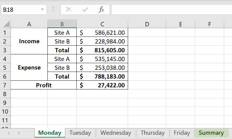
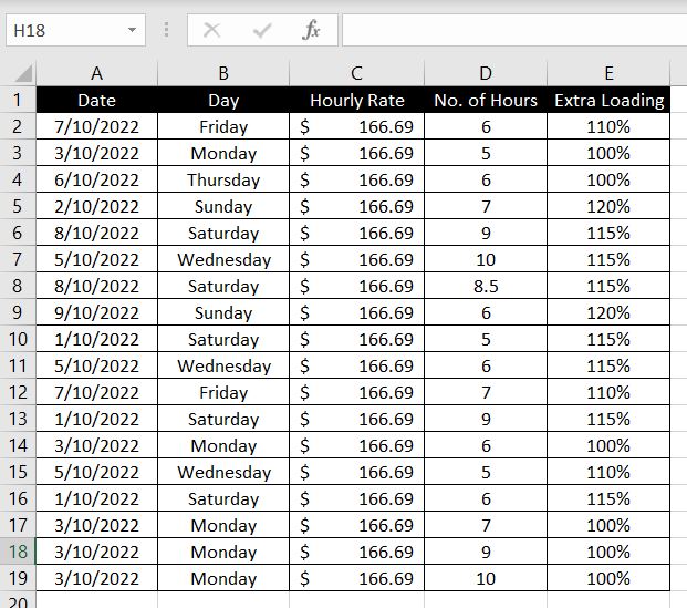
    Let’s use data below as an example:

    Excel-SUMIF-Data

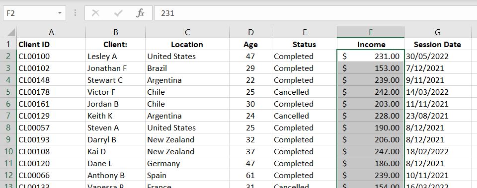
    With SUMIF function, we could do more insightful analysis such as getting total income based on location or total income for each year. We could basically separate data into groups. For example we could look at total income by age brackets of the clients.

    SUMIF-Basic-Example-Excel

    =SUMIF($C1:$C196,I2,$F1:$F196)

    In this example, we are adding income (sum_range – Column F) together if the location (range – Column C) matches our criteria (I2). In Cell I2, we have “United States”. Hence for every row where we have “United States” in Column C, Excel will add the income in Column F because the condition is met. And similarly for Brazil, Argentina and other locations.

    The good thing about SUMIF function is that it is not limited to the range column being on the left of the sum_range column. In the example above, we could easily have swapped Column C and Column F and SUMIF could still perform the exact same calculation for us.

    Numbers Not Adding Up Correctly? Important!

    Are values not adding up correctly? This, for obvious reason, is worse than getting an error. Why? Because it is not always obvious that we’ve made a mistake! This is why it is important to make sure we enter values into SUMIF function correctly, otherwise we could be getting an incorrect answer without even knowing it.

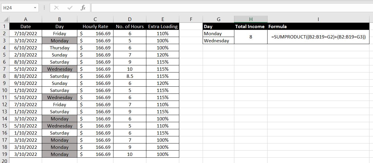
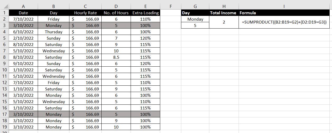
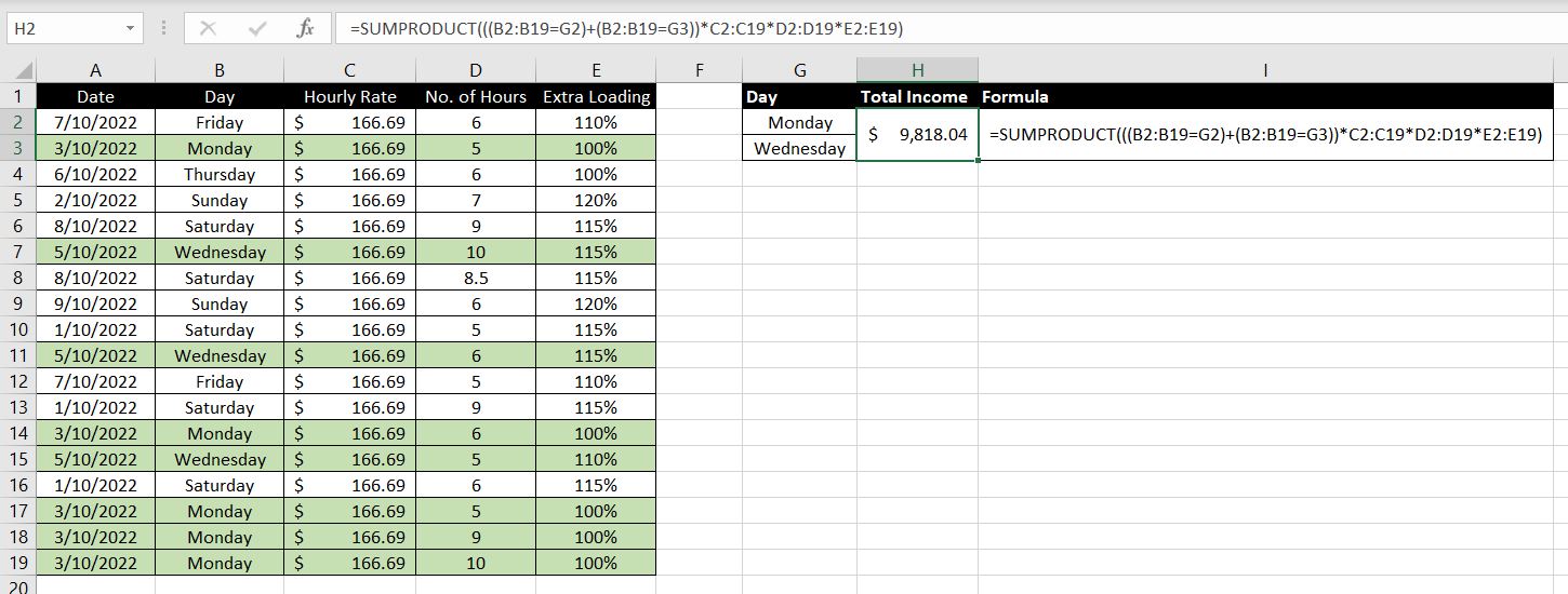
    With the SUMIF function, there are two arrays we need to enter: 1) range and 2) sum_range. It is very important that the two are aligned. Especially because of headings, it is easy to make a mistake and start one array in row one and the other in row 2. To clearly illustrate the problem and how the function works, we have changed the numbers and made the table smaller to make this more obvious:

    SUMIF-Numbers-Not-Adding-Up-Excel

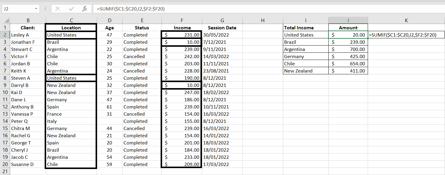
    =SUMIF($C1:$C20,I2,$F2:$F20)

    Notice that the range starts with Row 1 (C1) and sum_range starts with Row 2 (F2). Because of that, the corresponding rows do not match up anymore. From Excel’s perspective, the second and eighth rows in range C1:C20 are “United States”, hence it will return the second and eighth rows in sum_range F2:F20. But the second and eighth rows in F2:F20 are $10 and $10. Hence the SUMIF function returns $20 as the result.

    SUMIF with Dates and with Greater or Less Than

    So far we have only looked at examples where the criteria and values in range are exact matches. What if we don’t want an exact match? What if we want greater than (>) or less than (<)? Or what if we want to add up values across a certain period of time?

    Greater Than or Less Than…

    Let’s first look at how greater than and less than work in SUMIF functions. In this simple example, we will add up values in Income column if values in Age column is 1) over or equal 35 and 2) under 35:

    Excel-SUMIF-Greater-Than-Less-Than-Excel

    =SUMIF($D$2:$D$196,“>=”&35,$F$2:$F$196)

    =SUMIF($D$2:$D$196,“<“&35,$F$2:$F$196)

    Both are almost exactly the same except for the criteria. After all, both are looking at the same Age Column and the Income Column. In the first function, we want greater than or equal which is “>=”. And to connect that with 35, we just need to add a & in between.

    Similarly with the second formula, we want a less than which is “<“. And we connect it with &35. In this case we don’t want a “less than or equal to” because the “equal to” would overlap with the first “Over or equal 35” formula.

    Note: there are in fact some blank fields in the Age column but Excel would ignore them. To Excel, that means a blank cell is not the same as 0. With a “less than 35” condition, a blank cell is not considered meeting the condition. And in fact that would be perfect in our scenario, Column D is an Age column. A blank cell would more accurately be considered as “unknown, not 0.

    SUMIF with Dates

    Using very similar logic, we can add up values if the dates fall within a particular range. Here we want to add up values in Income column if Session Date is prior to 2022:

    SUMIF-Dates-Excel

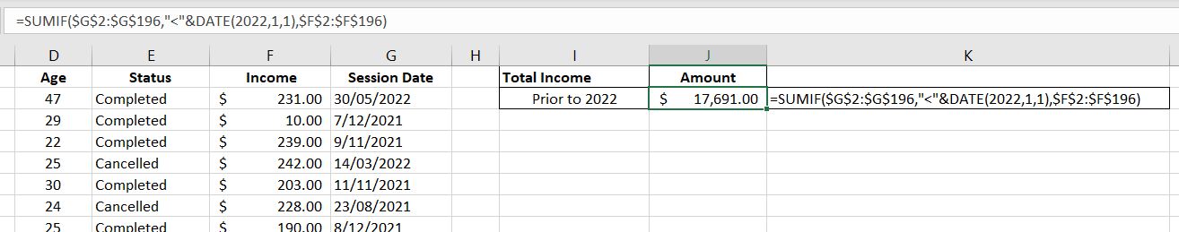
    =SUMIF($G$2:$G$196,“<“&DATE(2022,1,1),$F$2:$F$196)

    The range we are comparing the criteria with is G2:G196. The criteria is that the value in this range must be less than “<“ 01/01/2022 which is represented by DATE(2022, 1, 1) and we again connect the two with &. We could simply put it in a regular date format with quotation marks, e.g. “01/01/2022”. However because different countries could use different date formats (e.g. mm/dd/yyyy or dd/mm/yyyy), it will be less confusing to just use the DATE(year, month, date) function.

    Note: the good thing with SUMIF function with dates is that it knows to ignore blank cells in the range. That is if a cell is blank in G2:G196, it will NOT be considered as a condition met.

    Tip: always check your work. If the SUMIF function that is greater than or equal to a date and another SUMIF function that is less than that same date do not add up to the total, then you would know that there’s probably a field missing in the session date.

    SUMIFS – Multiple Conditions

    What if we want to add multiple conditions into SUMIF function? Well luckily there is a SUMIFS function. It is literally just a SUMIF but with multiple conditions. The order we enter our variables changes slightly. With SUMIFS, it is:

    = SUMIFS(sum_range, criteria_range1, criteria1, [critieria_range2, criteria2]…)

    Notice that there is no square bracket around sum_range now. This means sum_range is now a mandatory field. The first set of range and criteria is also mandatory. But conditions 2, 3, 4…are optional. Excel-SUMIFS-function-multiple conditions

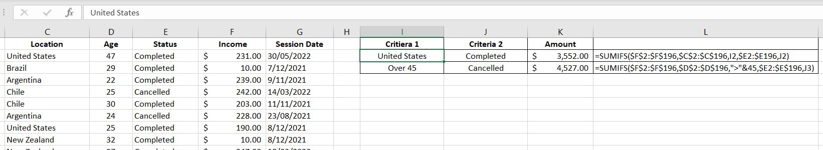
    =SUMIFS($F$2:$F$196,$C$2:$C$196,I2,$E2:$E196,J2)

    =SUMIFS($F$2:$F$196,$D$2:$D$196,”>”&45,$E2:$E$196,J3)

    The easiest way to visualize this is first we tell the function the range of cells which has the values we would like to add up (F2:F196). After that, we put in each set of criteria_range and the criteria:

    • In the first example, for Column C (Location), we are looking for “United States” as the criteria (Cell I2) and also in Column E (Status), we are looking for “Completed” as the criteria (Cell J2)
    • In the second formula, for Column D (Age), we are looking for values greater than 45 as the criteria and also in Column E (Status), we are looking for “Cancelled” as the criteria (Cell J3)

    Sum_Range Can Be Optional?

    Ever noticed that in the SUMIF function, sum_range is in square bracket? This would of course mean that this field is an optional input. The function can still work with or without this variable. Strange but it works.

    If the sum_range is blank, Excel will add up values in range field. That is, of course only if values in range are numerical values. We will show two examples below:

    1) Numerical Values

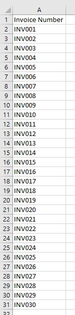
    Here’s a list of random number between 0 to 200 – randomly generated by RANDBETWEEN. In this example, we will add up the numbers if they are less than 100:

    SUMIF-Example-No-Sum_Range-Excel

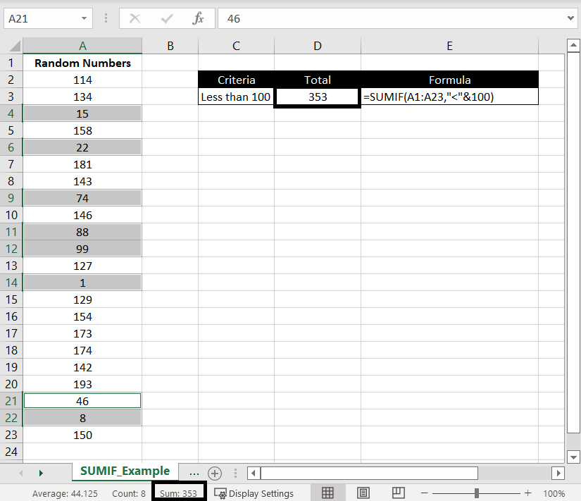
    =SUMIF(A1:A23,”<“&100)

    We highlighted cells with values less than 100 and we can see at the bottom the “Sum: 353” matches the SUMIF result. This shows that while the criteria is being matched against the range, values in the range would be added up.

    2) Non-Numerical Values

    Here we are doing a SUMIF in range A1:A23 and the criteria is “Dianne”:
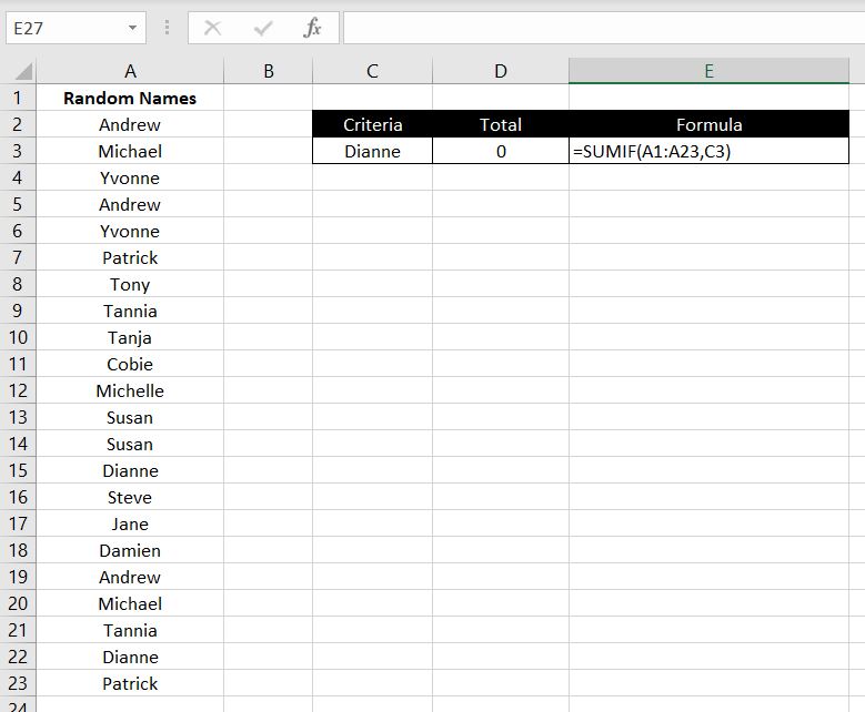
    SUMIF-No-Sum_Range-Names-Example-Excel

    =SUMIF(A1:A23,C3)

    Again no alert pop up appeared. Excel will happily calculate the function for us because sum_range is only an optional field. But as expected, because names are non-numerical values, there is nothing to add up. Hence the SUMIF function returns a 0.

    We hope you now have a good understanding of how SUMIF works in Excel. If you need any further clarification or if you feel that we’ve missed anything, please leave a comment below.

  • Split Texts in Cells Using Text To Columns

    Split Texts in Cells Using Text To Columns

    The reason why we all love Excel is because we have a lot of flexibility in formatting and manipulating data the way we want. Very often we are restricted by the systems we use in terms of how we can see and present our data. And this is why we export reports into Excel files and we can format data to the way we need them to be. For example we may need to separate a list of clients’ full names into first names and last names or we need to split a list of invoice numbers. In this article, we will explore different situations, various data types and different methods to split texts in cells.

    Text to Columns

    Text to Columns, as the name suggests, splits text in a cell (or a range of cells) into multiple adjacent columns.

    Text-to-Columns-Excel

    With Text to Columns, there are two options available:

    Excel-Text-to-Columns-Delimiter-Fixed-Width

    • Delimited: we can pick a particular character (symbol, letter or number) and every time Excel sees that character in the cell, it will split to the rest of the text into the next column. This could be useful with splitting full names into first names and last names by setting a space as the delimiter.
    • Fixed Width: we can split texts by setting break lines anywhere. E.g. we can choose to split texts at the fifth character in a cell. And we can create as many break lines as we want. So e.g. we can split texts at the fifth character, the seventh character and then the twentieth character. And as you can imagine, if we want to split full names into first names and last names, this would not be very useful because different names would have different numbers of characters.
    Tip: the purpose of Text to Columns is to split text across to adjacent cells. You will need to make sure the adjacent cells are empty otherwise you will get error message below:

    Text-to-Columns-Excel-Error

    Delimited

    With Text to Columns – Delimited, we can choose a character – any character we want (symbol, letter or number) and every time that character appears in the cell, Excel will split the text into another column. Here’s an example below:

    In our CRM, there’s a field which has checkboxes that allow more than one selection. And when we export the data into Excel, it’s formatted as below:

    Text-to-Columns-Excel-Delimited-Data

    The data is rather messy. For entries that have multiple selections, they are all entered into one cell. This makes it very hard to do any analysis.

    But we can also see that each selection is separated by a semi-colon (;). That means we can use Text to Columns – Delimited to separate each selection:

    1. Highlight Column A
    2. Select the Data tab at the top and click Text to Columns
      Text-to-Columns-Excel
    3. Select Delimited and click Next
    4. Select Semicolon
      Text-to-Columns-Excel-Delimited-Semi-Colon

      Note that here we could select “Other” and enter any character we want in the box next to it. The only limitation here is that although we can select multiple delimiters listed, only one character can be entered in the “Other” box.
    5. Click Next
    6. Click Finish

    And this will be the end result: Text-to-Columns-Excel-Delimited-Result

    It is now much easier to analyse the data e.g. using COUNTA or COUNTIFS.

    Here’s another example. When we copy and paste a table from PDFs to Excel, the format does not always transfer across the way we want it to:

    Text-to-Columns-Delimited-PDF-Data-Excel

    Of course we could use Power Query instead (see more here on Power Query) to export PDFs into Excel but we could also use Text to Columns with space as the delimiter. The result will not be 100% perfect (we will need to shift the headings a bit) but it will again be a lot easier to work with the data:

    Text-to-Columns-Delimited-PDF-Result-Excel

    With some copying and pasting, it will only take a minute or two before we can format it to a proper table:

    Text-to-Columns-Delimited-PText-to-Columns-Delimited-PDF-Result-Excel-FinalDF-Result-Excel-Final

    Fixed Width

    Text to Columns – Fixed Width gives us the choice to create break lines wherever we want – and as many as we want. Let’s take a look at the data below as an example. It is a list of invoice numbers and let’s say in this case, we want to separate “INV” and the invoice numbers:

    Text-to-Columns-Fixed-Width-Data-Excel

    In this case, Text to Columns – Delimited will not be very useful because there is nothing between “INV” and the invoice number. We could potentially use “V” as the delimiter. But you can see above in Delimiter section, when we use semicolon (;) as the delimiter, the semicolon disappears after the texts are split. This means if we use “V” as the delimiter, the end result will be “IN” and invoice number – “V” will disappear.

    The best way will be to use Text to Columns – Fixed Width:

    Text-to-Columns-Excel-Fixed-Width

    The line in between “INV” and the invoice number is the break line. And it can be inserted anywhere. In fact, we can insert more than one. We can insert as many break lines as we want. For example:

    Text-to-Columns-Excel-Fixed-Width-Many-Break-Lines

    And in this case, each character (“I”, “N”, “V”, “0”…) will be split into a separate cell

    But back to the example above, if we insert one break line between “INV” and the invoice number and we click “Finish”, we will get the following:

    Text-to-Columns-Fixed-Width-Data-Result-Excel

    In summary, there are pros and cons with using Delimited and Fixed Width. Which one you use depends on the data you currently have and how you want to split the text.

    As a final tip: we can see in the example above with Fixed Width, in using Text to Columns, we don’t necessarily have to select the whole column. Many reports we extract from systems have headings and we don’t want to split the headings. We can select the range of cells we want to split and apply Text to Columns only to those cells.

    If there’s anything else you would like us to add into this article, please leave a comment below! We would like to keep improving the content in our articles.

  • Generating Random Numbers in Excel

    Generating Random Numbers in Excel

    There could be a wide range of different reasons why generating random numbers could be useful in Excel. In this article, we will go through how to generate a random number in Excel, how to select a random value from a list or table and how to generate a random table of numbers.

    Generating a Random Number

    Random Number Within a Range

    To generate a random number, we can use the RANDBETWEEN function. With this function, we need to enter two variables – min and max. This sets the range which the random number must lie in between.

    RANDBETWEEN-Function-Excel

    Note that if we try to set a min that is a larger number than the max, we will get the #NUM error. But they can the same number. And if the min or max are not numbers, the RANDBETWEEN function will return with #VALUE. We can enter a decimal number for min and max but RANDBETWEEN will return a whole number (integer). Negative numbers work for min and max as well.

    Random Number In Multiples

    When we create random numbers, we often need to set parameters and limitations around what the numbers could be. In the section above, we know that RANDBETWEEN function allows us to set a range between which the number could lie. But we could also set additional parameters such generating numbers that are in multiples of 5s or 10s or 100s or the number must be an even number.

    We will do this by combining RANDBETWEEN function with the MROUND function. We have used the RANDBETWEEN function above. MROUND is an Excel built-in function that rounds a number to a specific multiple we specify. With this function, there are two variables we need to enter: 1) the number that requires rounding and 2) the multiple to which the number in 1) should round to. As a quick example:

    MROUND-example-Excel

    In this case, we’ve entered the number 49 and we want to round it to nearest multiples of 5. And the MROUND function returns the value of 50.
    Combining RANDBETWEEN and MROUND functions, we can first generate a random number within a specified range and then have the number rounded to a multiple we specify. In the example below, we will generate a number between 0 to 10000 and round it to multiples of 100:

    MROUND-RANDBETWEEN-Functions-Excel

    There is one thing to be careful with this:

    • It is possible for MROUND to round the random number to a number that is outside the range we specify in RANDBETWEEN

    As an example:

    MROUND-RANDBETWEEN-Functions-Outside-Range-Excel

    In this instance, we’ve set a range of 500 to 600 for RANDBETWEEN but because we are using MROUND to round the result to nearest thousand, Excel has returned a result of 1000. Conversely if we set the range to be 0 to 499 and MROUND with 1000 multiple, Excel will always guarantee to return the result of 0.

    Random Decimal Between 0 and 1

    There’s a built-in function in Excel which allows users to a random decimal number between 0 to 1. It is the RAND function. This function requires no variable input. To use this function, simply enter “=RAND()”:

    RAND-Function-Excel

    We could then use the ROUND function to specify how many decimal places we want from this RAND function. For example we could specify to only want 3 decimal places for this number:

    ROUND-RAND-Functions

    Generating a Table of Random Numbers

    To generate an array of random numbers, there is an Excel built-in function called RANDARRAY. There are 5 variables that could be entered.

    1. Row
    2. Column
    3. Min
    4. Max
    5. Integer/Decimal

    They’re all optional as you can tell with the square brackets. And by default if we just enter “=RANDARRAY()”, Excel will generate one number between 0 to 1 and it will be a decimal. This means by default, without entering any variables RANDARRAY and RAND are very much the same. But of course by giving us the option to enter the 5 fields, we can do a lot more with this function.

    In the example below, we will create a 3 by 4 table of random numbers between 10 to 100 and they’re all integers:

    RANDARRAY-Excel

    Generating a Random Number (Bigger Than One)…With Decimals

    So far we’ve gone through the RAND function, the RANDBETWEEN function and the RANDARRAY function. The limitation between RAND and RANDBETWEEN is that RAND only generates a number between 0 to 1 and RANDBETWEEN only generates whole numbers (integers). What if we want to generate a decimal number but larger than one?

    We can use the RANDARRAY function. But instead of creating an array or a table, we will set the function to generate a 1 row by 1 column array:

    Generate-Decimal-Number-Bigger-Than-One-Excel

    In this case, we’ve set row and column to 1 which means only one number will be generated. We’ve then set the range (min and max) for which the number to be generated. Lastly, we specified that we want the number generated to be a decimal number.

    And of course similar to sections above, we could combine this with the ROUND function to specify how many decimal places we want. Or if generating integers, we could use MROUND function to round the number to the nearest multiple of our choice.

    Selecting a Random Text from a List/Table

    In the Index and Match – A More Advanced Lookup article, we went through how to use the INDEX and MATCH functions to look up a value. In summary, an INDEX function allows us to search for an item or a value in an array of data, given a specific row number and a column number. Given the section above, we can generate a random number with the RANDBETWEEN function and also set a range as to where the number needs to lie in between. This means we can use RANDBETWEEN to generate a random row number and/or column number in the INDEX function.

    In this case we have a list of names in Column A:

    Name-Column-Excel

    To use INDEX function to return “Daniel M”, we could do “=INDEX(A1:A20, 17, 1)”. This is because “Daniel M” is row 17 in the A1:A20 range and in Column A – first column. But suppose we don’t want “Daniel M” to be returned and we want to have a random person, we can replace “17” with a RANDBETWEEN function:

    Select-Random-From-List-Excel

    =INDEX(A1:A20, RANDBETWEEN(2,20), 1)

    In this case, we are using RANDBETWEEN function to generate a random number between 2 to 20. The reason why 1 is not the minimum is because Cell A1 is “Staff” and that is only a heading so we don’t want that returned from the INDEX function.

    This also works when data is not in a single column but in a table. In the example above, we’ve set the column number to 1. But we can set another RANDBETWEEN for the column number. We just need to be careful with setting the min and max for each. In the example below, the table goes from row 2 to 7 hence the function is RANDBETWEEN(2, 7). And it goes across three columns hence column number is RANDBETWEEN(1, 3).

    Select-Random-From-Table-Excel

    And this is how we can select a cell randomly from a list or from a table.

    In this article we have gone through how to generate random numbers and set parameters on the numbers. This includes requiring the numbers to fall within a particular range and rounding the random number to its nearest multiples. We also went through how to generate a table/list of random numbers and also how to randomly select a value from a list or a table. If there is anything else you would like us to include in this article, please leave a comment below!

  • INDEX and MATCH – A More Advanced Lookup in Excel

    INDEX and MATCH – A More Advanced Lookup in Excel

    In the VLOOKUP article, we have looked at some limitations with the VLOOKUP function in Excel. For example, we must start from the leftmost column and look up values on the righthand side. Similarly with HLOOKUP, we must start from the top row and look for values downwards. So if you are looking for a more flexible formula in Excel, INDEX and MATCH functions could be your solution. And they are simple to use. First we will go through the INDEX and MATCH functions separately and then we will explore how they can be used together to do a lookup.

    Index Function

    The purpose of the INDEX Function in Excel is to:

    • Look through an array of data and given a specific row number and a column number, it will return a specific value in that array of data
    • =INDEX(Array of data, Row Number, Column Number)

    Let’s have a look at the example below. Here we are looking into the A1:C14 array of data and specifically, we want the data in Row 5 and Column 3:

    Index-Function-Excel

    =INDEX(A1:C14, 5, 3)

    Match Function

    The purpose of the MATCH Function in Excel is to:

    • Look through a row/column of data and given a lookup value, it will return where the location of that lookup value is
    • =MATCH(lookup value, row/column of data, [match type])

      [match type]: similar to VLOOKUP or HLOOKUP, we need to specify whether we want an exact match. 0 is TRUE. 1 is FALSE.

    Let’s have a look at the example below. Here we are looking into the array A1:A14 and specifically, we want to know where “Daniel H” is:

    • =MATCH(E5, A1:A14,0)

    Match-Function-Excel

    And as we can see, “Daniel H” is in Row 7 and is 7th down the row from A1.

    Index Match Functions

    Now let’s put the two together. As mentioned above, the INDEX function is:

    • =INDEX(Array of data, Row Number, Column Number)

    We could now replace the row number or column number (or both) with a MATCH function. Remember, the MATCH function returns the position of a lookup value in a row or column. Once we have the position of the lookup value in a row (or column), we can also specify the column number (or row number) and the INDEX function will return the corresponding value in the array of data.

    Example:

    Index-Match-Function-Excel

    =INDEX(A1:C14, MATCH(E5, A1:A14, 0), 3)

    =INDEX(A1:C14, MATCH(E8, C1:C14, 0), 1)

    For the first example, we want to find the Employee Number for “Daniel H”. We could easily use the VLOOKUP function (=VLOOKUP(E5, A1:C14, 3, FALSE)). But INDEX and MATCH can work perfectly as well. First we use MATCH function to look up “Daniel H” in A1:A14. This will return 7 as Daniel H is 7th down the list. The INDEX function then becomes =INDEX(A1:C14, 7, 3). 7th row and 3rd column, this will be “EMP0006”.

    One thing VLOOKUP will not be able to do though is the second example – working from right to left. In this case, we have “EMP0002” and we want to find who the employee is. First we use the MATCH function to look up “EMP0002” along C1:C14. This will return 3 as EMP0002 is 3rd down the list. The INDEX function then becomes =INDEX(A1:C14, 3, 1). 3rd row and 1st column, this will be “Susan W”.

    It works just as well if we replace column number with MATCH function:

    Index-Row-Match-Excel

    =INDEX(A1:C14, 8, MATCH(E5, A1:C10))

    In this case, we want to find “June” amount for Darrin W. Let’s say we already know that Darrin W is in row 8, we then use MATCH function to find “June” across A1:C1 (“=MATCH(E5, A1:C1, 0)). This will return 2 as June is second across the row. The INDEX function becomes =INDEX(A1:C14, 8, 2). 8th row and 2nd column is “$8000”.

    Index Match Match Function

    Even better, we could replace both row number and column number in the INDEX function with MATCH functions:

    Index-Match-Match-Excel

    Let’s break this down:

    • =INDEX(A1:F14, MATCH(H5,A1:A14,0),MATCH(I5,A1:F1,0))

      Row Number – MATCH(H5, A1:A14, 0): this is to search for “Nathan M” along A1:A14. This will return 5
    • Column Number – MATCH(I5, A1:F1,0): this will search for “May” along A1:F1. This will return 4.
    • Hence the INDEX function is equivalent to =INDEX(A1:F14, 5, 4). Row 5, Column 4 is “$2500”.

    Common Errors

    We will now look at some of the common errors with Index & Match functions:

    • #VALUE: we cannot put in a negative number for row number or column number. This just wouldn’t make sense.
    • #REF: when the row number or column number we specified is bigger than the array of data. E.g. with array A1:C5, it would mean there could only be 3 columns. If we specify a column number that is 4 or bigger, INDEX will return #REF.
    • Make sure the “array of data” in both INDEX and MATCH function are aligned: this requires more attention because we will not get an Excel error in this case. But the value returned will be incorrect:

      Excel-Index-Match-Function-Wrong-Value-Excel

      Notice that the returned value is $2000, not $2500. The reason is that the MATCH function is looking at A2:A7 array whereas INDEX function is looking at A1:F14 array. The MATCH function looking for “Nathan M” in A2:A7 means the function will return a value of 4. This means the INDEX function has now become =INDEX(A1:F4, 4, 4). Row 4, Column 4 is $2000.

    We hope you now understand how INDEX and MATCH functions work and common errors to look out for. Feel free to leave a comment if we’ve missed anything or if you have any feedback on this article!

  • IF Function with Multiple Conditions

    IF Function with Multiple Conditions

    In this article, we will explore how IF function works in Excel. It is simple but very effective and useful. We will also explore how to add multiple conditions in an IF function. First we will explain how an IF function works, then we will go on to combine IF function with AND and OR functions. And at the end we will also look at nested IF functions.

    IF Function

    The IF function in Excel allows us to:

    • Have Excel examine a logical test. And if the test returns TRUE, we can have the function return a particular value which we get to specify. Alternatively if the test returns FALSE, we can have the function return another value which we also gets to specify.

    The function is:

    • =IF(logical test, [value if true], [value if false])

    The square brackets around value if true and value if false do mean they are optional fields. The function will still work if nothing is entered for those two fields. In that case, TRUE will return 0 and FALSE will return FALSE.

    Here’s an example below. We have a list of clients’ ages but the data is very hard to be presented because we could have data ranging from around 5 to 85. Using a simple IF function, we can group clients’ ages into “minor” or “adults”:

    If-function-Excel

    Now we can use a COUNTIF function on column B to calculate the number of adults and minors in this list.

    Value If True and Value If False

    With [value if true] and [value if false], we have set a string for each in the example above. However we can make it dynamic and have a formula there too. Here’s a simple example:

    If-function-formula-Excel

    The formula we have in C2 is:

    • =IF(B2=”Cancelled”, $F$3, VLOOKUP(A2,$E$5:$F$9,2,FALSE))

    Explanation: We first have Excel check the status in Column B. If status is “Cancelled”, the logical statement will be TRUE hence F3 – Cancellation Fee of $75 will populate. If the status is not “Cancelled”, Excel will use VLOOKUP to search for the price in the Price Guide in E5:F9 for the relevant program in Column A.

    What Logical Tests Can We Include?

    In the example above, we used “less than” as the logical test but there are so many more we could do in Excel. It would be impossible to list them all down but to list a few, we could:

    • = : to compare two values
    • < or >: “less than” or “greater than”
    • <= or >=: “less than or equal to” or “greater than or equal to”
    • ISBLANK: if a cell is blank
    • ISNUMBER: if the value in a cell is a number
    • ISTEXT: if the value in a cell is a text – note that if the value is a number or date, it will return FALSE

    IF & AND Functions

    Essentially with IF functions, we enter a logical test and if it is TRUE, the [value if true] will return. Alternatively [value if false] will return. With the AND function, we can add multiple conditions into the logical test. And the logical test will only return TRUE if all conditions are met. As an example:

    IF-AND-Functions-Excel

    • =IF(AND(A2<>”Saturday”, A2<>”Sunday”),”Working Day”, “Weekend”)

    Explanation: in this case, two conditions must be met, the cell on the left must not be (<>) “Saturday” and must not be “Sunday”. If both conditions are met, “Working Day” will populate. Otherwise it will be “Weekend”. And of course you can add more than 2 conditions into the AND functions.

    IF & OR Functions

    The OR function is very similar, except only one of the conditions needs to be met for the logical test to return TRUE. Let’s explore the same scenario above but this time we will use the OR function to reach the same outcome:

    If-OR-Functions-Excel

    • =IF(OR(A2=”Saturday”, A2=”Sunday”), “Weekend”, “Working Day”)

    Explanation: in this case, only one of the logical tests in the OR function needs to be TRUE. That is, if the cell on the left is “Saturday” OR “Sunday”, the cell will be populated with “Weekend”. Otherwise it will be “Working Day”. And again, we can add more than 2 logical tests in OR functions.

    Nested IF Functions

    So far we’ve only looked at IF functions with two possible outcomes. If TRUE then [value if true] will appear. If FALSE then [value if false] will appear. Things are not always so simple. What happens if you have more than 2 possible outcomes? Consider this example below:

    If a staff is employed on a casual basis, there will be no bonus. There will also be no bonus if no KPIs are met. If one of the two KPIs are met and the staff is employed on a permanent basis, a Tier 2 bonus will be rewarded. And finally if both KPIs are met and the staff is employed on a permanent basis, a Tier 1 bonus will be rewarded:

    Excel-Nested-If-bonus-Table

    Excel-Nested-IF-Functions

    Let’s break down this long formula:

    • =IF(OR(A2=”Casual”, AND(B2=”Not Met”,C2=”Not Met”)),”No bonus”, IF(AND(B2=”Met”, C2=”Met”),”Tier 1 Bonus”, “Tier 2 Bonus”))
    • =IF(OR(A2=”Casual”, AND(B2=”Not Met”,C2=”Not Met”)),”No bonus” : If staff is a casual OR if both KPIs are not yet, Excel will return “No bonus”. If this is not TRUE, then Excel will move onto the next IF function:
      • IF(AND(B2=”Met”, C2=”Met”),”Tier 1 Bonus”, “Tier 2 Bonus”)): If the first logical test was not met then it would already mean that the employee is not a casual staff and the employee met one or both of the KPIs. In this next IF function, if both KPIs are met, Excel will return “Tier 1 Bonus”. Otherwise it would mean only one of the KPIs in which case “Tier 2 Bonus” will return.

    Nested IFs, AND and OR functions

    As shown above with the AND and OR functions, we can sometimes reach the same outcome with either functions. We can also use nested IF functions to reach the same result. But imagine how many times we would have to nest the IF functions when we could perhaps group all conditions into an OR function. The question to ask is how many possible outcomes there are. If there are more than two, you will most likely need to use nested IF functions. But if there are only two possible outcomes, you should most likely be able to group all the conditions into AND and OR functions.

    Please feel free to leave a comment below if there’s more you would like us to go through in this topic!

  • User-Defined Functions – Writing Your Own Functions in Excel

    User-Defined Functions – Writing Your Own Functions in Excel

    There are over 500 built-in functions in Excel but yet you may have trouble finding one that suits your need. Are there calculations that you do on a regular basis over and over again? And you are tired of typing in that same formula in again and again every time. You can save time by writing your very own user-defined functions in Excel.

    Before we start, we need to make sure the Developer tab is enabled in Excel. If you don’t see a Developer tab at the top, it’s simple – have a look at How To Enable Macro/Visual Basic for Application (VBA):

    Developer-tab-enabled-Excel

    If you can see the Developer tab, then let’s get started! We will first go through a simple example of creating a function that calculates the area of a circle. And then we will go through another example which is more complex and uses a loop.

    Creating Your Very Own Functions

    1. Open Visual Basics

    You can open Visual Basics by going to Developer Tab > Visual Basics:

    Open-vba-developer-tab-excel

    Or you can press Alt + F11.

    2. Create a New Module

    At the top, click on Insert > Module:

    Create-new-module-vba-excel

    3. Name of Function and Required Field(s)

    3.1. Unique Name for the Function

    Now it’s time to think of a unique name for the function and what variables or fields should be required. It is best practice to give the function a name that is relevant to its purpose. For example, it’ll be very confusing to others who use the spreadsheet if you name the function “Bob”. And it’ll be confusing for yourself. A few months later you might come back and wonder what the function “Bob” is supposed to calculate. In this example we will create a user-defined function that calculates the area of a circle so we will call the function “AreaOfCircle”.

    You also want the name to be unique. Because Excel already has over 500 built-in functions, you won’t want one that is already used by Excel. In fact, if you do, your user-defined functions will not work. Excel’s built-in existing functions will take place over your user-defined functions.

    3.2. Variables and Fields

    Technically not every function requires variables. It probably won’t be of much use but you can create a function that returns a constant value every time. For example you can leave the variables blank and have the function AreaOfCircle = 2 in the module. In which case, AreaOfCircle() will always return 2. But for example if we want to calculate area of a rectangle then the variables will be length and width.

    In this scenario, what variables are required in order to calculate the area of a circle? Since A = πr2, the only variable is r – the radius. In the empty module, enter the following:

    Public Function Name of your Function (variable1, variable 2…)

    End Function

    And in our case:

    Creating-UDF-Excel

    Public Function AreaOfCircle (radius)

    End Function

    4. Write Your Formula and Calculation

    This is of course the crux of the function. What is your function? What would you like Excel to calculate for you with this new function? To stick with our example above, we want to calculate the area of a circle:

    Area-of-circle-UDF-function-Excel

    We first set a new article x to be the value of Pi. And then we set AreaOfCircle to equal x * radius ^ 2 which is equivalent to A = πr2. In this case we set x as Pi.

    Public Function AreaOfCircle (radius)

    x = Application.WorksheetFunction.Pi

    AreaOfCircle = x * radius ^ 2

    End Function

    5. Let’s Check Our Work!

    Go back to our Excel sheet. Click on any cell and start typing “=” and the name of your function. You should be able to see it:

    Checking-UDF-Excel-Functions

    Once you see that your function is there, let’s check the calculation. The easiest way is to use this function in one cell and then put in the exact same formula in the cell underneath it manually with the same variable(s). Check out below:

    Testing-UDF-function-Excel

    The results are the same which is good. Test out a few more variables to make sure the function is working as intended.

    6. (Optional) Setting Variables Using IF Statements

    Now that our function is working, is there a way to improve it? This part is optional. Depending on what your function is, in most cases there should be parameters around what your variables could be. For example in some cases, the variables should only be integers. And in the case of a circle, the radius should only be a positive number. It can be a decimal but it certainly does not make sense to have a negative radius.

    To do this:

    Before defining the AreaOfCircle function, add an IF function. If the radius variable entered is less than 0, the function will return “Invalid variable entered”. In all other situations, calculate the area of circle.

    Public Function AreaOfCircle(radius)

    If radius < 0 Then

    AreaOfCircle = “Invalid variable entered”

    Else:

    x = Application.WorksheetFunction.Pi
    AreaOfCircle = x * radius ^ 2

    End If

    End Function

    Invalid-Variable-UDF-function-module-Excel

    Invalid-Variable-UDF-function-Excel

    In these cases, notifying the user an invalid variable was entered would most likely be more useful than actually calculating the area of circle with a negative 1 radius.

    Now let’s move onto a more complex example which involves a loop in the user-defined function

    Creating a User-Defined Function with Loop

    When we were writing the article for COUNT functions, it got us wondering if, given a specified range of cells, there was a way to count the number of cells containing data that has more than x number of characters inside. Well let’s write our own:

    Public Function CountLen(cellrange, character)

    Dim c As range

    x = 0

    For Each c In cellrange

    If Len(c) > character Then

    x = x + 1

    End If

    Next c

    CountLen = x

    End Function

    UDF-function-with-loop-Excel

    To put this into words:

    • We’ve called this new function “CountLen” and there are two variables required by the user every time: 1) the range of cells to count in (cellrange) 2) how many characters should be in the cell in order for the function to count the cell as meeting the condition (character)
    • First we create a new variable x and we set it as 0 at first. And for each cell in the range of cells specified (cellrange), if the number of character is greater than what we’ve specified in the second variable (character) then Excel will add 1 to x every time. After all the cells have been looped through, CountLen will return the value of x.

    Here’s an example below. In A2:A15, we’ve entered a bunch of random data. Let’s test this out with different variables to check if our function is working. Note that in the function, we’ve decided to set the function to check if the number of characters in each cell is greater than second variable specified, not greater than or equal to. Hence if we set the second variable as 2, Excel will only count if the number of characters is 3 or more:

    Testing-UDF-Loop-Function-Excel

    To check our results, we created Column B which counts the number of characters in corresponding cell in Column A with the LEN function. There are 11 cells in A2:A15 that have more than one character in them, and there are 6 cells in A2:A15 that have more than 3 characters in them.

    Are there any user-defined functions you need help with and want us to go through? Let us know in the comment below and we will keep add to our article to make it more complete.